Random Variables

The first step to understand random variable is to do a fun experiment. Go outside in front of your house with a pen and paper. Take note of every person you pass and their hair color & height in centimeters. Spend about 10 minutes doing this.

Congratulations! You have conducted your first experiment! Now you will be able to answer some questions such as:

How many people walked past you?
Did many people who walked past you have blue hair?
How tall were the people who walked past you on average?

You pass 10 people in this experiment, 3 of whom have blue hair, and their average height may be 165.32 cm. In each of these questions, there was a number; a measurable quantity was attached.

Definition

A random variable rv is a real-valued function, whose domain is the entire sample space of an experiment. Think of the domain as the set of all possible values that can go into a function. A function takes the domain/input, processes it, and renders an output/range. This set of real values obtained from the random variable is called its range.

A random variable (rv) is a function that maps events (from the sample space S) to the real numbers. It’s a function which performs the mapping of the outcomes of a random process to a numeric value.

The domain of a random variable is a sample space, which is represented as the collection of possible outcomes of a random event. For instance, when a coin is tossed, only two possible outcomes are acknowledged such as heads or tails.

Denoted by

Random variables Denote by a capital letters near the end of the alphabet (e.g. X, Y ).

Note

Why is it called a random variable?
Because we think of it as a variable that take random value intuitively. Formally they are function.

Probability Distribution

A Probability Distribution is a graph, table, or function that gives the probability for each value of the random variable.

Requirments

The sum of the probabilities is 1. $\sum f(x)=1 $.
Every probability $p_i$ is a number between 0 and 1. $ 0 \leq f(x) \leq 1$

Difference between random variables and probability distributions

A random variable is a numerical description of the outcome of a statistical experiment. The probability distribution for a random variable describes how the probabilities are distributed over the values of the random variable.

Types of Random Variables

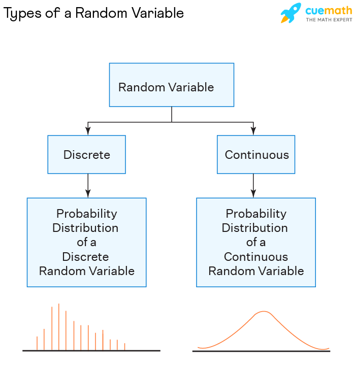
Discrete random variable: A discrete random variable is a type of random variable that has a countable number of distinct values that can be assigned to it, such as in a coin toss.
Continuous random variable: A continuous random variable stands for any amount within a specific range or set of points and can reflect an infinite number of potential values, such as the average rainfall in a region.

Big Picture In statistics, we will model populations using random variables (e.g. mean, variance) of these random variables will tell us about the population we are studying.

Probability mass function (P.M.F)

The probability that a discrete random variable $X$ takes on a particular value $x$ that is $P(X=x)$ is denoted by

\[ \text{p.m.f } \large = f(x) = f_x(x) = f_y(y) \]

Properties

The probability mass function, $P(X=x)=f(x)$, of a discrete random variable $X$ is a function that satisfies the following properties:

All of the probabilities must be positive. $P(X=x)=f(x)>0$, if $x \in$ the support $S$
Sum of all probabilities of same sample space equals to 1. $\sum_{x \in S} f(x)=1$
$P(X \in A)=\sum_{x \in A} f(x)$

$\text{Random variable}=X= \begin{cases} 1, & \text { if "Heads" } \\ 0, & \text { if "Tails" } \end{cases} = \begin{cases} P(X=1), & \text { if "Heads" } \\ P(X=0), & \text { if "Tails" } \end{cases}$

$PMF=f(x)=f_x(x)=P(X=x)= \begin{cases}1 / 2, & \text { if } x=0 \\ 1 / 2, & \text { if } x=1 \\ 0, & \text { otherwise }\end{cases}$

\[ p(x)=P(X=x)=P(\text { all } x \in S \mid X(s)=x) \]

Interview Question

Q: Let $f(x)=c x^{2}$ for $x=1,2,3$. Determine the constant $c$ so that the function $f(x)$ satisfies the conditions of being a probability mass function?

Answer: Using property no 2

\[\begin{split} \begin{aligned} \sum_{x=1}^{3} f(x) &=\sum_{x=1}^{3} c x^{2}=c \sum_{x=1}^{3} x^{2} \\ &=c\left[1^{2}+2^{2}+3^{2}\right]=c[1+4+9] \\ &=c(14) \stackrel{\text { set }}{=} 1 = c=1/14 \\ f(x) &=\frac{1}{14} x^{2} \text { for } x=1,2,3 \end{aligned} \end{split}\]

Cumulative distribution function (CDF)

The cumulative distribution function (CDF or cdf) of the random variable X has the following definition:

\[ F_X(t) = P(X \leq t) = \sum_{x \leq y} P(X=t) = \int_{-\infty}^{t} f(t)dt \]

Properties

The cdf of random variable X has the following properties:

The cdf, $F_{X}(t)$, ranges from 0 to 1 . This makes sense since $F_{X}(t)$ is a probability.
If $X$ is a discrete random variable whose minimum value is $a$, then $F_{X}(a)=P(X \leq a)=P(X=a)=f_{X}(a)$. If $c$ is less than $a$, then $F_{X}(c)=0$.
If the maximum value of $X$ is $b$, then $F_{X}(b)=1$.
Also called the distribution function.

Example

Suppose X is a discrete random variable. Let the pmf of X be equal to

\[ f(x)=\frac{5-x}{10}, \quad x=1,2,3,4 \]

Suppose we want to find the cdf of $X$. The cdf is $F_{X}(t)=P(X \leq t)$.

For $t=1, P(X \leq 1)=P(X=1)=f(1)=\frac{5-1}{10}=\frac{4}{10}$.
For $t=2, P(X \leq 2)=P(X=1$ or $X=2)=P(X=1)+P(X=2)=\frac{5-1}{10}+\frac{5-2}{10}=\frac{4+3}{10}=\frac{7}{10}$
For $t=3, P(X \leq 3)=\frac{5-1}{10}+\frac{5-2}{10}+\frac{5-3}{10}=\frac{4+3+1}{10}=\frac{9}{10}$.
For $t=4, P(X \leq 4)=\frac{5-1}{10}+\frac{5-2}{10}+\frac{5-3}{10}+\frac{5-4}{10}=\frac{10}{10}=1$.

Probability density function (PDF)

X = f(x) is the probability density function of the continues random variable X.

\[ P(a \leq X \leq b)=\int_{a}^{b} f(x) d x \]

f(x) = Curve under which area represent the probability $P(a \leq X \leq b)=\int_{a}^{b} f(x) d x$

Expected Value (Mean or Average)

The concept was first devised in the 17th century to analyze gambling games and answer questions such as:

How much do I gain - or lose - on average, if I repeatedly play a given gambling game?
How much can I expect to gain - or lose - by making a certain bet?

For example, if you play a game where you gain 2$ with probability 1/2 and you lose 1$ with probability 1/2, then the expected value of the game is half a dollar

\[ 2$ \times \frac{1}{2} + (-1$) \times \frac{1}{2} = \frac{1}{2} $ = 0.5$ \]

it means that if you play this game many times, and the number of times each of the two possible outcomes occurs is proportional to its probability, then on average you gain 1/2$ each time you play the game.

Definition

The expected value or mean of a random variable is a weighted average of all possible outcomes. In the case of a continuum of possible outcomes, the expectation is defined by integration.

Denoted by $\mu_x$ or $E(X)$.

\[ \large \mu=\mu_x=E(X)=\sum_{x} k P(X=x) = \int_{-\infty}^{\infty} x f(x) d x \]

Example

5 exams result : 70 +80 + 80 + 90 + 90

$Avg = \frac{70+80+80+90+90}{5} = \frac{1}{5}(70)+\frac{2}{5}(80)+\frac{2}{5}(90) = 82.5 $

Let X represent the outcome of a roll of a fair six-sided die. The possible values for X are 1, 2, 3, 4, 5, and 6, all of which are equally likely with a probability of $1/6$ The Expected Value of X is

$E[X] = 1\cdot\frac16 + 2\cdot\frac16 + 3\cdot\frac16 + 4\cdot\frac16 + 5\cdot\frac16 + 6\cdot\frac16 = (1+2+3+4+5+6) / 6= 3.5$

x	1	2	3
P(X=x)	1/4	1/4	1/2

$E[X] =(1)(1 / 4)+(2)(1 / 4)+(3)(1 / 2) = 9/4 = 2.25 = \sum_{x} x P(X=x)$

Imagine a game in which, on any play, a player has a 20% chance of winning $3 and an 80% chance of losing $1. The probability mass function of the random variable , the amount won or lost on a single play is:

\[\begin{split} x \quad $3 \quad -$1 \\ f(x) \quad 0.2 \quad 0.8 \end{split}\]

so the average amount won (actually lost, since it is negative)

\[ E(X)=(\$ 3)(0.2)+(-\$ 1)(0.8)=\$-0.20 \]

In the long run you guaranteed to lose no more than 20 cents.

Pytorch implementation

import torch

# Create a tensor
T = torch.Tensor([2.453, 4.432, 0.754, -6.554])
print("T:", T)

# Compute the mean and standard deviation
mean = torch.mean(T)
print("mean:", mean)

T: tensor([ 2.4530,  4.4320,  0.7540, -6.5540])
mean: tensor(0.2713)

import matplotlib.pyplot as plt
import seaborn as sns

sns.set_theme(style="darkgrid")
data = torch.randn(25)

print(data)

print("Mean :", torch.mean(data))

_ =sns.displot(data,kde=True, )
plt.axvline(torch.mean(data), color='green')
plt.show()

tensor([ 0.1304, -0.2829,  0.7720,  0.6261, -0.7537, -0.6111,  0.0727,  0.8777,
        -0.0064,  0.5796, -1.1902, -1.0818, -0.8887, -0.9166, -0.3301,  1.7974,
        -0.0081,  0.1470, -1.2143, -1.8930, -0.6445,  1.4764, -0.4136,  0.1353,
        -0.3242])
Mean : tensor(-0.1578)

../_images/f43f15fa252304d1158fa33476ff794a6bbb799bb2d01ed1f1304f9aa9a98caa.png

Properties

Expectation is a linear operator, which means for our purposes it has a couple of nice properties.

Expected value of a constant

A perhaps obvious property is that the expected value of a constant is equal to the constant itself.

\[ \large E[c] = c \]

\[\begin{split} \begin{gather} \large \text{Proof}\\ E[2] = \sum_{x} k P(X=x) = \sum_{x} 2 P(X=x) \\ = 2 \sum_{x} P(X=x) = 2 \times 1 \\ = 2 \end{gather} \end{split}\]

Scalar multiplication of a random variable

If X is a random variable and a is a constant, then

\[ E[aX] = aE[X] \]

\[\begin{split} \begin{gather} \large \text{Proof}\\ E[2X] = \sum_{x} 2 k P(X=x) = 2 \sum_{x} k P(X=x) \\ = 2 E[X] \\ \end{gather} \end{split}\]

Expectation of a product of random variables

Let X and Y be two random variables. In general, there is no easy rule or formula for computing the expected value of their product. However, if X and Y are statistically independent, then

\[ E[XY] = E[X]E[Y] \]

Expectation of a sum of random variables

\[ E(X+Y)=E(X)+E(Y) \]

If random variables is function

\[\begin{split} E(g(X))=\left\{\begin{array}{l} \sum_{k} g(k) P(X=k), X \text { is discrete } \\ \int_{-\infty}^{\infty} g(x) f(x) d x, X \text { is continuous. } \end{array}\right. \end{split}\]

$E(a X+b)=\sum_{k}(a X+b) P(X=k)$

$E(a X+b)= a \sum_{k} k P(X=k)+b \sum_{k} P(X=k)$

$E(a X+b)= a E(x) + b * 1 = a E(x) + b$

Law of the Unconscious Statistician

IF X with pdf $f_x(x)$ and g is a function Find 𝖤[𝗀(𝖷)]

Let Y=g(X). The pdf for Y is:

$f_{Y}(y)=f_{X}\left(g^{-1}(y)\right) \cdot\left|\frac{d}{d y} g^{-1}(y)\right| = \text { So, } E[g(X)]=E[Y]=\int_{-\infty}^{\infty} y \cdot f_{Y}(y) d y$

$=\int_{-\infty}^{\infty} y \cdot f_{x}\left(g^{-1}(y)\right) \cdot\left|\frac{d}{d y} g^{-1}(y)\right| d y$

$\text { Let } x=g^{-1}(y) \text {. Then } d x=\frac{d}{d y} g^{-1}(y) d y$

$E[g(X)]=\int_{-\infty}^{\infty} g(x) f_{X}(x)) d x$

Variance

Measures how far we expect our random variable to be from the mean.
Measures of spread of a distribution.
Variance is a measure of dispersion.

Denoted by

\[ \large \sigma^2 \text{ or } V(X). \]

\[ V(X) = E[(X - E[X])^2] = E[(X - \mu)^2] = E[X^2] - E[X]^2 \]

To better understand the definition of variance, we can break up its calculation in several steps:

Compute the expected value of $X$, denoted by $\mathrm{E}[X]$.
Construct a new random variable $Y=X-\mathrm{E}[X]$ equal to the deviation of $X$ from its expected value.
Take the square $ Y^{2}=(X-\mathrm{E}[X])^{2} $ which is a measure of distance of $X$ from its expected value (the further $X$ is from $\mathrm{E}[X]$, the larger $\left.Y^{2}\right)$
Finally, compute the expectation of $Y^{2}$ to know the average distance:

\[ \mathrm{E}\left[Y^{2}\right]=\mathrm{E}\left[(X-\mathrm{E}[X])^{2}\right]=\operatorname{Var}[X] \]

From these steps we can easily see that

variance is always positive because it is the expected value of a squared number.
the variance of a constant variable $X$ (i.e., a variable that always takes on the same value) is zero; in this case, we have that $X=\mathrm{E}[X], Y^{2}=0$ and $\mathrm{E}\left[Y^{2}\right]=0$
the larger the distance $Y^{2}$ is on average, the higher the variance.

\[\begin{split} \begin{gather} \large \text{Proof} \\ V(X) = E[(X - \mu)^2] \\ V(X) = E[X^2 - 2\mu X + \mu^2] \\ V(X) = E[X^2 - 2\mu E[X] + \mu^2] \\ V(X) = E[X^2 - 2\mu^2 + \mu^2] \\ V(X) = E[X^2 - \mu^2] \\ V(X) = E[X^2] - E[X]^2 \end{gather}\end{split}\]

For continuous rv

If X is a continuous random variable, the variance is defined by the integral of the probability density function. $V(X)=\int_{-\infty}^{\infty} (x - \mu_x)^2 f(x) d x$

$V(X)=\int_{-\infty}^{\infty} (x - \mu_x)^2 f(x) d x$

$= \int_{-\infty}^{\infty}\left(x^{2}-2 \mu_{x} x+\mu_{x}^{2}\right) f(x) d x$

$= \int_{-\infty}^{\infty}x^{2} f(x) d x - 2 \mu_{x} \int_{-\infty}^{\infty}x f(x) d x + \mu_{x}^{2} \int_{-\infty}^{\infty}f(x) d x$

$V(X) = E(X^2)-E(X)^2$

Properties

Addition to a constant

Let $a \in \mathbb{R}$ be a constant and let $X$ be a random variable.

\[ Var[a+X]=Var[X] \]

Thanks to the fact that $\mathrm{E}[a+X]=a+\mathrm{E}[X]$ (by linearity of the expected value), we have

\[\begin{split} \begin{aligned} \operatorname{Var}[a+X] &=\mathrm{E}\left[(a+X-\mathrm{E}[a+X])^{2}\right] \\ &=\mathrm{E}\left[(a+X-a-\mathrm{E}[X])^{2}\right] \\ &=\mathrm{E}\left[(X-\mathrm{E}[X])^{2}\right] \\ &=\operatorname{Var}[X] \end{aligned} \end{split}\]

Multiplication by a constant

Let $a \in \mathbb{R}$ be a constant and let $x$ be a random variable.

\[ Var[a X]=a^{2} Var[X] \]

Thanks to the fact that $E[a X]=a E[X]$ (by linearity of the expected value), we obtain

\[\begin{split} \begin{aligned} Var[a X] &=E\left[(a X-E[a X])^{2}\right] \\ &=E\left[(a X-a E[X])^{2}\right] \\ &=\mathrm{E}\left[a^{2}(X-\mathrm{E}[X])^{2}\right] \\ &=a^{2} \mathrm{E}\left[(X-\mathrm{E}[X])^{2}\right] \\ &=a^{2} \operatorname{Var}[X] \end{aligned} \end{split}\]

Find Var[aX] = ?

Let Y = aX. Then, $\mu_y = E[Y] = E[aX] = E[a\mu_x] = aE[\mu_x] = aE[X]$

==> $Var[aX] = Var[Y] = Var[(Y - \mu_y)^2] = a^2 Var[(X - \mu_x)^2] = a^2 V(X)$

For Function

$V(g(X))= \begin{cases}\sum_{k}(g(k)-E(g(X)))^{2} P(X=k), & X \text { discrete } \\ \int_{-\infty}^{\infty}(g(x)-E(g(X)))^{2} f(x) d x, & X \text { continuc }\end{cases}$

Find V(a X+b)

$V(a X+b)=E[(a X+b-E(a X+b))^2]$

$= E[(a x+ \not{b} -a E(x)- \not{b})^2]$

$= E[(a^2 (x - E(x))^2]$

$= a^2 E[(x - E(x)^2] = a^2 V(x)$

Variance measure the spread the data B shift the data but doest not affect the spread.

Find Var[aX]

Let Y=aX. Then

\[\begin{split} \mu_{Y}=E[Y]=E[a X]=a E[X]=a \mu_{X} \\ Var[aX]=Var[Y]=E\left[\left(Y-\mu_{Y}\right)^{2}\right] \\ =a^{2} E\left[\left(X-\mu_{X}\right)^{2}\right] \\ =a^2 Var[X] \end{split}\]

Find Var[X + Y]

\[\begin{split} Var[X+Y]=Var[X]+Var[Y] \\ \end{split}\]

We will see that this is true if X and Y are independent.
Need concept of “covariance”.

Standard Deviation

The standard deviation is the square root of the variance. $\sigma_x = \sqrt{V(X)}$

Indicator function

The indicator function of an event is a random variable that takes

value 1 when the event happens;
value 0 when the event does not happen.

Let A = Set of real numbers

\[\begin{split} I_{A}(x)= \begin{cases}1, & \text { if } x \in A \\ 0, & \text { if } x \notin A\end{cases} \end{split}\]

Other definition

The indicator function of a subset A of a set X is a function.

$\text{Indicator function}_{A}(X) = \mathbf{1}_A(x) =\begin{cases} 1, & \text { if } A \cap X \neq \emptyset \\ 0, & \text { otherwise }\end{cases}$

Notation= $\mathbb{1} _{A}(x)$

Random Sample

A collection of random variables is independent and identically distributed if each random variable has the same probability distribution as the others and all are mutually independent.

\[ \large \text{Random Sample} = $X_1, X_2, X_3, ..., X_n \]

Suppose that $X_1, X_2, X_3, ..., X_n$ is a random sample from the Normal distribution with parameters $\mu$ and $sigma^2$. Mu and sigma are same for all random variables

\[ X_{1},X_{2}, \ldots, X_{n} \stackrel{\mathrm{iid}}{\sim} N(\mu, \sigma^{2}) \]

Suppose that $X_1, X_2, X_3, ..., X_n$ is a random sample from the gamma distribution with parameters $alpha$ and $\beta$.

\[ X_{1},X_{2}, \ldots, X_{n} \stackrel{\mathrm{iid}}{\sim} \Gamma(\alpha, \beta) \]

Example

A good example is a succession of throws of a fair coin: The coin has no memory, so all the throws are independent. And every throw is 50:50 (heads:tails), so the coin is and stays fair - the distribution from which every throw is drawn, so to speak, is and stays the same: identically distributed.

Independent and identically distributed random variables (IID)

Random Sample == IID