What is Machine Learning?
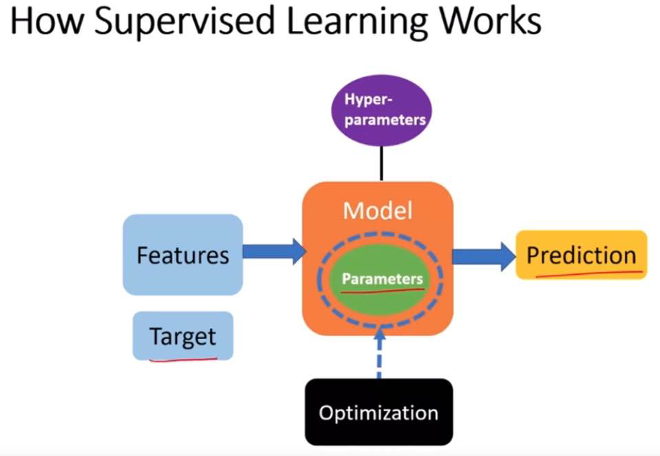
Statistical learning is about using many tools to understand data. These tools can be grouped into two types: supervised and unsupervised. Supervised learning means you create a model to predict or estimate an outcome based on inputs. This kind of problem is found in many areas like business, medicine, space science, and government policies. Unsupervised learning means you don’t have a specific outcome you’re looking for, but you still try to find patterns or relationships in the data.
Best book on Machine Learning
My notes are based on this book reference. https://www.statlearning.com/
Simple Linear Regression
Simple linear regression is a method used in statistics to model the relationship between two variables by fitting a linear equation to observed data. One variable is considered to be an explanatory variable (independent variable), and the other is considered to be a dependent variable. The linear regression aims to draw a straight line that best fits the data by minimizing the sum of the squares of the vertical distances of the points from the line.
Formula
The equation of a simple linear regression line is:
where:
y is the dependent variable,
x is the independent variable,
\(\beta_0\) is the y-intercept of the regression line,
\(\beta_1\) is the slope of the regression line, which indicates the change in y for a one-unit change in x,
\(\epsilon\) is the error term (the difference between the observed values and the values predicted by the model).
The goal is to estimate the coefficients \(\beta_0\) and \(\beta_1\) that minimize the sum of squared residuals (the differences between the observed values and the values predicted by the model).
For example, X may represent TV advertising and Y may represent sales. Then we can regress sales onto TV by ftting the model
\(\beta_0\) and \(\beta_1\) are two unknown constants that represent he intercept and slope terms in the linear model. Together, \(\beta_0\) and \(\beta_1\) are known as the model coefficients or parameters. Once we have used our raining data to produce estimates \(\hat{\beta}_0\) and \(\hat{\beta}_1\) for the model coefficients, we can predict future sales on the basis of a particular value of TV advertising sy computing
where \(\hat{y}\) indicates a prediction of \(Y\) on the basis of \(X=x\). Here we use a hat symbol, ‘ , to denote the estimated value for an unknown parameter or coefficient, or to denote the predicted value of the response.
Estimating the Coefcients
In practice, \(\beta_0\) and \(\beta_1\) are unknown. So before we can use to make predictions, we must use data to estimate the coefficients. Let $\( \left(x_1, y_1\right),\left(x_2, y_2\right), \ldots,\left(x_n, y_n\right) \)$
represent \(n\) observation pairs, each of which consists of a measurement of \(X\) and a measurement of \(Y\). In the Advertising example, this data set consists of the TV advertising budget and product sales in \(n=200\) different markets. (Recall that the data are displayed in Figure 2.1.) Our goal is to obtain coefficient estimates \(\hat{\beta}_0\) and \(\hat{\beta}_1\) such that the linear model (3.1) fits the available data well-that is, so that \(y_i \approx \hat{\beta}_0+\hat{\beta}_1 x_i\) for \(i=1, \ldots, n\). In other words, we want to find an intercept \(\hat{\beta}_0\) and a slope \(\hat{\beta}_1\) such that the resulting line is as close as possible to the \(n=200\) data points. There are a number of ways of measuring closeness. However, by far the most common approach involves minimizing the least squares criterion, and we take that approach in this chapter. Alternative approaches will be considered in Chapter 6.
Let \(\hat{y}_i=\hat{\beta}_0+\hat{\beta}_1 x_i\) be the prediction for \(Y\) based on the \(i\) th value of \(X\). Then \(e_i=y_i-\hat{y}_i\) represents the \(i\) th residual - this is the difference between the \(i\) th observed response value and the \(i\) th response value that is predicted by our linear model. We define the residual sum of squares (RSS) as $\( \mathrm{RSS}=e_1^2+e_2^2+\cdots+e_n^2 \)$
Example 1: Height and Weight
Imagine we have data on the heights and weights of a group of people. We could use simple linear regression to predict the weight of someone based on their height. In this example:
The independent variable \(x\) would be height (e.g., in centimeters).
The dependent variable \(y\) would be weight (e.g., in kilograms).
By analyzing the data, we calculate the values of \(b_0\) (the intercept) and \(b_1\) (the slope).
Suppose we find the regression equation to be \(y = 50 + 0.5x\). This means that for every additional centimeter in height, we expect the weight to increase by 0.5 kilograms, starting from 50 kilograms.
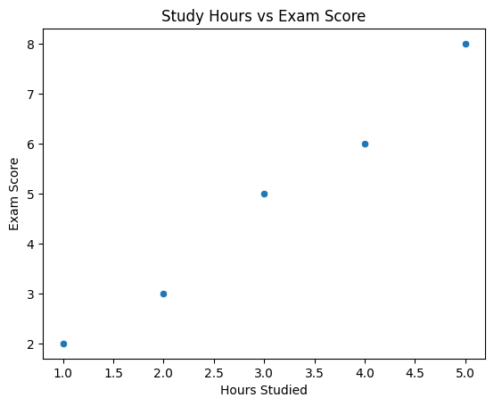
Example 2: Hours spent studying vs. Exam score
First, we can visualize the data to understand its distribution and the relationship between x and y
import seaborn as sns
import matplotlib.pyplot as plt
import pandas as pd
import numpy as np

# Sample data: Hours spent studying vs. Exam score
data = {
    'Hours_Studied': [1, 2, 3, 4, 5],
    'Exam_Score': [2, 3, 5, 6, 8]
}
df = pd.DataFrame(data)

# Plotting the data
sns.scatterplot(data=df, x='Hours_Studied', y='Exam_Score')
plt.xlabel('Hours Studied')
plt.ylabel('Exam Score')
plt.title('Study Hours vs Exam Score')
plt.show()
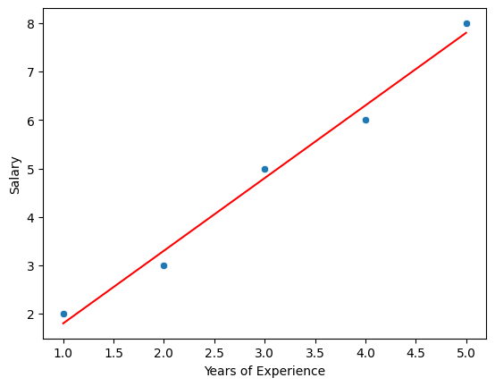
beta_1, beta_0 = np.polyfit(df.Hours_Studied, df.Exam_Score, 1)
# Print the computed parameters
print(f"Slope: {beta_1}, Intercept: {beta_0}")

regression_line = beta_0 + beta_1 * df.Hours_Studied

# Plot original data points
sns.scatterplot(x=df.Hours_Studied, y=df.Exam_Score)

# Plot regression line
plt.plot(df.Hours_Studied, regression_line, color='red')

plt.xlabel('Years of Experience')
plt.ylabel('Salary')
plt.show()
Slope: 1.4999999999999998, Intercept: 0.3000000000000001
import torch
import torch.nn as nn
import torch.optim as optim

# Preparing the data
X = torch.tensor(df['Hours_Studied'].values, dtype=torch.float32).view(-1, 1)
Y = torch.tensor(df['Exam_Score'].values, dtype=torch.float32).view(-1, 1)

# Defining the linear regression model
model = nn.Linear(in_features=1, out_features=1)

# Loss function and optimizer
criterion = nn.MSELoss()
optimizer = optim.SGD(model.parameters(), lr=0.01)

# Training the model
epochs = 500
for epoch in range(epochs):
    # Zero the gradients
    optimizer.zero_grad()

    # Forward pass
    outputs = model(X)
    loss = criterion(outputs, Y)

    # Backward and optimize
    loss.backward()
    optimizer.step()

    if (epoch+1) % 100 == 0:
        print(f'Epoch [{epoch+1}/{epochs}], Loss: {loss.item()}')

# Coefficients
print('Estimated coefficients:')
print('Weight:', model.weight.item())
print('Bias:', model.bias.item())
Epoch [100/500], Loss: 0.06318604946136475
Epoch [200/500], Loss: 0.06161843612790108
Epoch [300/500], Loss: 0.06082212179899216
Epoch [400/500], Loss: 0.06041758134961128
Epoch [500/500], Loss: 0.06021212413907051
Estimated coefficients:
Weight: 1.4905762672424316
Bias: 0.33402296900749207
Optmization
In simple linear regression, the Least Squares Method is used to find the values of the coefficients \(\beta_0\) and \(\beta_1\) that minimize the sum of the squared differences between the observed values and the values predicted by the linear model. The sum of squared differences, also known as the sum of squared residuals (SSR), is given by:
where \(y_i\) are the observed values, \(\hat{y_i}\) are the predicted values, and \(n\) is the number of observations. The predicted values are calculated using the linear model equation:
To find the values of \(\beta_0\) and \(\beta_1\) that minimize the SSR, we take the partial derivatives of the SSR with respect to \(\beta_0\) and \(\beta_1\), set them equal to zero, and solve the resulting system of equations. This process is called the method of least squares.
Derivatives Calculation
Partial Derivative with Respect to \(\beta_0\):
Using the chain rule, this derivative simplifies to:
Partial Derivative with Respect to \(\beta_1\):
This derivative simplifies to:
Solving for \(\beta_0\) and \(\beta_1\)
To find the values of \(\beta_0\) and \(\beta_1\) that minimize the SSR, we set each derivative equal to zero:
\( -2 \sum_{i=1}^{n} (y_i - \beta_0 - \beta_1x_i) = 0 \)
\( -2 \sum_{i=1}^{n} x_i(y_i - \beta_0 - \beta_1x_i) = 0 \)
These can be simplified and rearranged to form a system of linear equations:
\( \sum_{i=1}^{n} y_i = n\beta_0 + \beta_1\sum_{i=1}^{n} x_i \)
\( \sum_{i=1}^{n} x_iy_i = \beta_0\sum_{i=1}^{n} x_i + \beta_1\sum_{i=1}^{n} x_i^2 \)
Solving this system of equations gives the values of \(\beta_0\) and \(\beta_1\):
Interpretation
\(\beta_1\) (the slope) represents the estimated change in the dependent variable (\(y\)) for a one-unit change in the independent variable (\(x\)).
\(\beta_0\) (the intercept) represents the estimated value of \(y\) when \(x = 0\).
This method ensures that the line of best fit is determined by minimizing the difference between the observed values and the values predicted by the linear model, specifically by minimizing the sum of the squares of these differences.
Evaluating the Model
In linear regression, the evaluation of the model’s performance often involves determining how well the model fits the observed data. Two key metrics used in this context are the Residual Sum of Squares (RSS) and the Total Sum of Squares (TSS). Understanding these metrics allows us to assess the proportion of the variance in the dependent variable that is predictable from the independent variable.
Residual Sum of Squares (RSS)
The Residual Sum of Squares (RSS), also known as the Sum of Squared Residuals (SSR), measures the amount of variance in the dependent variable that is not explained by the regression model. In simpler terms, it quantifies how much the data points deviate from the regression line. Mathematically, RSS is defined as:
where:
\(y_i\) is the actual value of the dependent variable for the \(i\)th observation,
\(\hat{y_i}\) is the predicted value of the dependent variable for the \(i\)th observation based on the regression line,
\(n\) is the total number of observations.
A smaller RSS indicates a model that closely fits the data.
Total Sum of Squares (TSS)
The Total Sum of Squares (TSS) measures the total variance in the dependent variable. It represents how much the data points deviate from the mean of the dependent variable. TSS is an indicator of the total variability within the data set. It is defined as:
where:
\(y_i\) is the actual value of the dependent variable for the \(i\)th observation,
\(\bar{y}\) is the mean value of the dependent variable across all observations.
TSS is used as a baseline to compare the performance of the regression model.
The relationship between RSS and TSS is crucial for understanding how well the linear regression model fits the data. To quantify this, one common metric is the \(R^2\) statistic, also known as the coefficient of determination. \(R^2\) measures the proportion of the variance in the dependent variable that is predictable from the independent variable(s). It is calculated as:
An \(R^2\) value of 1 indicates that the regression model perfectly fits the data (with RSS = 0).
An \(R^2\) value of 0 suggests that the model does not explain any of the variability in the dependent variable around its mean (with RSS = TSS).
While \(R^2\) is a useful indicator of model fit, it’s important to consider other metrics and tests as well, especially when dealing with multiple regression models or models that might be overfitting the data.
Coefficient Significance
The significance of a coefficient in a linear regression model indicates whether a variable has a statistically significant relationship with the dependent variable. It’s assessed using the t-test, which evaluates the null hypothesis that the coefficient is equal to zero (no effect) against the alternative hypothesis that the coefficient is not equal to zero (a significant effect).
T-statistic is calculated as:
where \(\hat{\beta_j}\) is the estimated coefficient for the predictor variable \(j\), and \(SE(\hat{\beta_j})\) is the standard error of the estimated coefficient.
The t-statistic is compared against a critical value from the t-distribution with \(n-p-1\) degrees of freedom, where \(n\) is the number of observations and \(p\) is the number of predictors. If the absolute value of the t-statistic is greater than the critical value, the null hypothesis is rejected, indicating that the coefficient is statistically significant.
Example: Imagine a dataset where we’re predicting house prices based on various features. One of the features is the number of bedrooms. Suppose the estimated coefficient for the number of bedrooms is 20,000 (indicating that each additional bedroom is associated with an average increase of $20,000 in house price), with a standard error of 5,000.
Assuming a critical value of 2.576 for a 99% confidence level, the t-statistic is greater than the critical value, suggesting the number of bedrooms is a significant predictor of house price.
Test Error
Test error, also known as the mean squared error (MSE) on the test set, measures the model’s performance on unseen data. It’s calculated by comparing the model’s predictions on the test set with the actual values.
where \(n_{\text{test}}\) is the number of observations in the test set, \(y_i\) are the actual values, and \(\hat{y_i}\) are the predicted values by the model.
The MSE provides a numeric measure of the average squared deviation between the observed actual outcomes and the outcomes predicted by the model. A lower MSE indicates a better fit of the model to the data.
Example: Continuing with the house price prediction model, suppose we have a test set of 100 houses. After predicting the prices with our model, we calculate the differences between the actual prices and the predicted prices, square those differences, and average them. If the resulting MSE is \(10,000,000, this means, on average, the model's predictions deviate from the actual prices by about \)3,162 (the square root of MSE) per house.
Both the significance of coefficients and test error provide valuable insights into a linear regression model’s effectiveness and reliability. Coefficient significance helps identify which variables have a meaningful impact on the dependent variable, while test error quantifies the model’s predictive accuracy on new, unseen data.
Multi-Linear Regression
Multi-linear regression is an extension of simple linear regression to predict an outcome based on multiple predictors or independent variables. The goal of multi-linear regression is to model the relationship between two or more predictors and a response variable by fitting a linear equation to observed data. The formula for a multi-linear regression model can be expressed as:
Where:
\(Y\) is the dependent variable (the variable being predicted),
\(X_1, X_2, ..., X_n\) are the independent variables (predictors),
\(\beta_0\) is the intercept,
\(\beta_1, \beta_2, ..., \beta_n\) are the coefficients of the predictors which represent the weight of each predictor in the equation,
\(\epsilon\) is the error term, the part of \(Y\) the regression model is unable to explain.
Multi-Linear Regression in PyTorch
PyTorch is a popular open-source machine learning library for Python, primarily used for applications such as computer vision and natural language processing. It’s also extensively used for deep learning applications, but you can certainly use it for simple multi-linear regression.
Here’s a basic example of how to implement multi-linear regression in PyTorch:
Data Preparation: First, we need to prepare our dataset. This involves splitting our data into predictors (X) and a target variable (Y).
Model Creation: We’ll create a linear model using PyTorch’s
nn.Linearmodule to represent our multi-linear regression model.Loss Function: The loss function will measure how well the model predicts the target variable. For regression problems, Mean Squared Error (MSE) is commonly used.
Optimizer: This is what we’ll use to update the model parameters (\(\beta\) values) to minimize the loss function. A common optimizer is Stochastic Gradient Descent (SGD).
Example Code
This code snippet demonstrates a simple example of performing multi-linear regression using PyTorch. Here, X is our matrix of predictors, and Y is the target variable. We define a model with nn.Linear specifying 3 input features and 1 output feature. The training loop updates our model’s weights using the specified optimizer and loss function. After training, we print the loss at every 100 epochs to observe how it decreases, indicating that our model is learning. Finally, we print out the learned parameters, which are the weights and bias from our model.
Remember, this is a very basic example. In practice, you’d have a much larger dataset, you would divide your data into training and test datasets, and you might need to normalize your data for better performance.
import torch
import torch.nn as nn
import torch.optim as optim

# Example dataset with 3 predictors
X = torch.tensor([[1, 2, 3], [4, 5, 6], [7, 8, 9], [10, 11, 12]], dtype=torch.float32)
Y = torch.tensor([[14], [32], [50], [68]], dtype=torch.float32)  # target variable

# Define the model
model = nn.Linear(in_features=3, out_features=1)

# Loss function
criterion = nn.MSELoss()

# Optimizer
optimizer = optim.SGD(model.parameters(), lr=0.01)

# Training loop
epochs = 100
for epoch in range(epochs):
    # Forward pass: Compute predicted y by passing x to the model
    Y_pred = model(X)

    # Compute loss
    loss = criterion(Y_pred, Y)

    # Zero gradients, perform a backward pass, and update the weights.
    optimizer.zero_grad()
    loss.backward()
    optimizer.step()

    if (epoch+1) % 50 == 0:
        print(f'Epoch {epoch+1}, Loss: {loss.item()}')

# Display learned parameters
for name, param in model.named_parameters():
    if param.requires_grad:
        print(name, param.data)
Epoch 50, Loss: inf
Epoch 100, Loss: inf
weight tensor([[-4.2858e+35, -4.8812e+35, -5.4765e+35]])
bias tensor([-5.9534e+34])
Bias-Variance Trade-Off
The Bias-Variance Trade-Off is a fundamental concept in supervised machine learning that describes the trade-off between the ability of a model to approximate the true underlying function (bias) and its sensitivity to fluctuations in the training data (variance). Understanding this trade-off is crucial for building models that generalize well from training data to unseen data.
Bias
Bias refers to the error due to overly simplistic assumptions in the learning algorithm. High bias can cause the model to miss relevant relations between features and target outputs (underfitting), meaning the model is not complex enough to capture the underlying patterns in the data.
Variance
Variance refers to the error due to too much complexity in the learning algorithm. High variance can cause the model to model the random noise in the training data (overfitting), meaning the model is too complex and captures noise as if it were a pattern in the data.
Trade-Off
The trade-off is that algorithms with high bias typically have lower variance, and vice versa. A model with high bias might overly simplify the model, making it perform poorly on both training and unseen data. A model with high variance might perform exceptionally well on training data but poorly on unseen data because it’s too tailored to the training data, including its noise.
Ideally, you want to find a sweet spot that minimizes both bias and variance, providing good generalization to new data.
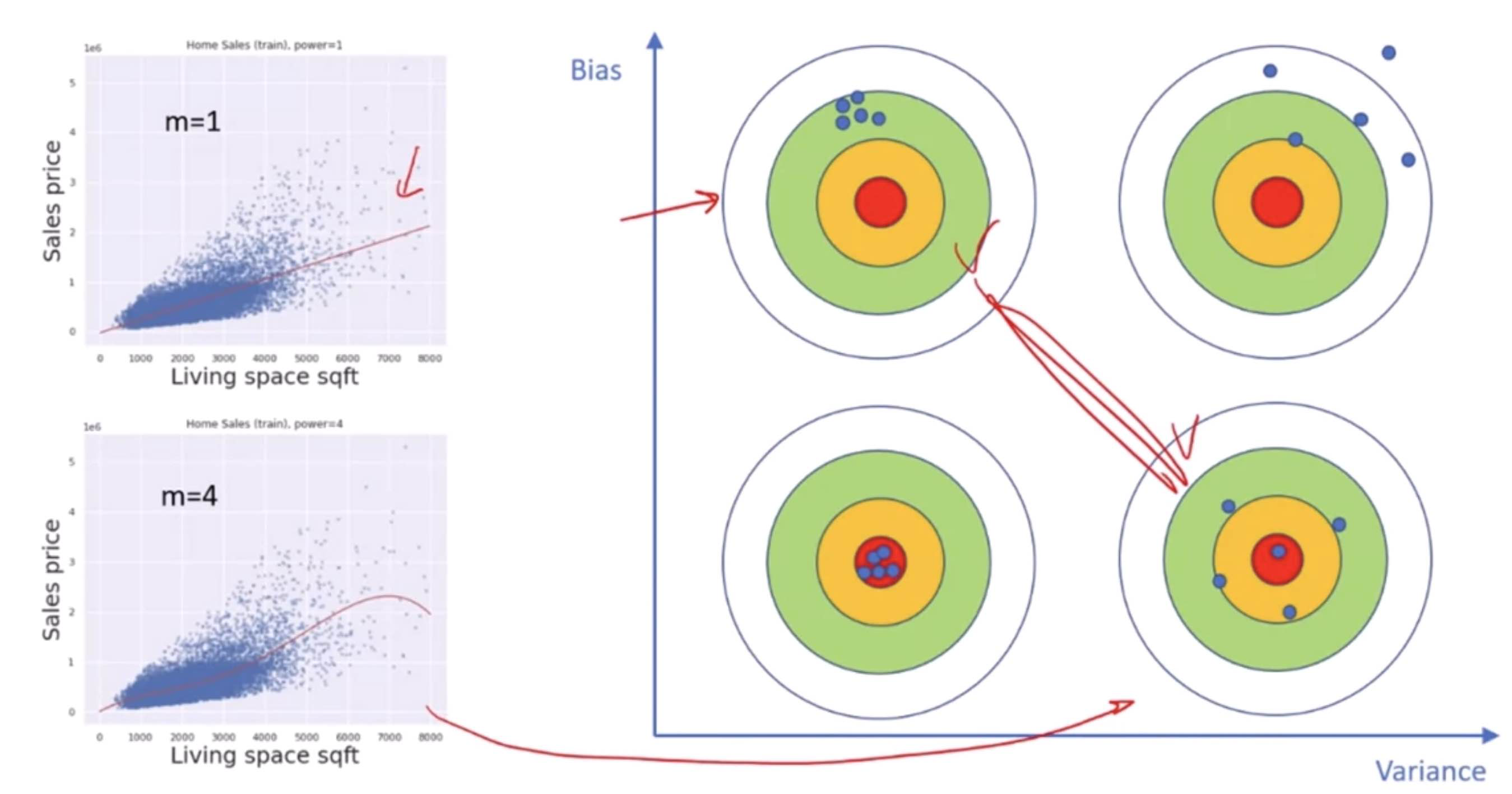
Image Examples
Let’s illustrate this with some image examples.
High Bias (Underfitting): Imagine a scenario where you’re trying to fit a line (linear regression) through data points that clearly form a curved pattern (quadratic). The linear model is too simple to capture the curve, resulting in high bias.
High Variance (Overfitting): Now, imagine fitting a high-degree polynomial through those same points. The model fits the training data points perfectly, including the noise, resulting in a wavy line that doesn’t capture the true underlying pattern.
Bias-Variance Tradeoff: The optimal model would be one that correctly assumes a quadratic relationship, fitting a curve that captures the underlying pattern without being affected by the noise.
Let’s generate these examples visually.
High Bias Example: A straight line attempting to fit through quadratic data points.
High Variance Example: A high-degree polynomial line that passes through every point, including noise.
Ideal Model: A quadratic curve that fits well with the underlying pattern of the data, avoiding overfitting and underfitting.
I’ll create an image to represent the concept of the Bias-Variance Tradeoff visually.
The image above visually represents the Bias-Variance Tradeoff in machine learning. It consists of three panels, each illustrating a key concept:
High Bias: The first panel shows a simple straight line that does not capture the essence of the underlying curve formed by the data points. This scenario is typical of models with high bias, where the simplicity of the model prevents it from capturing the true relationship between variables, leading to underfitting.
High Variance: The second panel depicts a highly complex, wavy line that passes through every single data point, including noise. This is characteristic of models with high variance, where the complexity of the model causes it to capture noise as if it were a significant pattern, leading to overfitting.
Ideal Model: The third panel illustrates an optimal curve that smoothly captures the general pattern of the data points without fitting to the noise. This represents the desirable balance in the Bias-Variance Tradeoff, where the model is complex enough to capture the underlying pattern but not so complex that it fits the noise in the data.
This visualization aids in understanding the trade-off between bias and variance, highlighting the importance of finding a model that achieves a good balance for optimal performance on unseen data.
Types of variables in multi linear regression