Decision Tree
Decision trees are a type of supervised learning algorithm used for both classification and regression tasks, though they are more commonly used for classification. They are called “decision trees” because the model uses a tree-like structure of decisions and their possible consequences, including chance event outcomes, resource costs, and utility.
How Decision Trees Work
The algorithm divides the data into two or more homogeneous sets based on the most significant attributes making the groups as distinct as possible. It uses a method called “recursive partitioning” or “splitting” to do this, which starts at the top of the tree (the “root”) and splits the data into subsets by making decisions based on feature values. This process is repeated on each derived subset in a recursive manner called recursive partitioning. The recursion is completed when the algorithm cannot make any further splits or when it reaches a predefined condition set by the user, such as a maximum tree depth or a minimum number of samples per leaf.

Components of Decision Trees
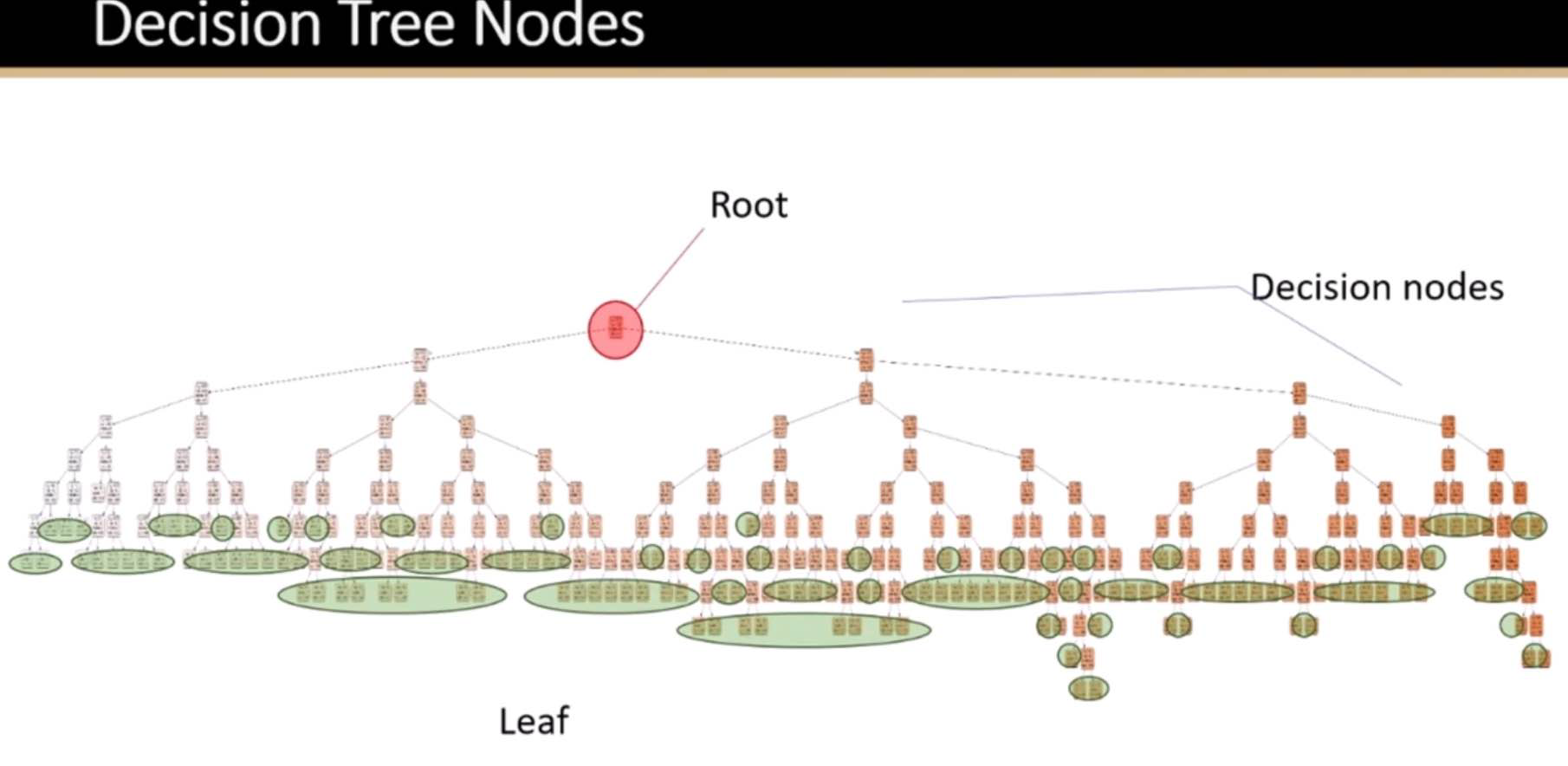
Root Node: Represents the entire dataset, which gets divided into two or more homogeneous sets.
Splitting: Process of dividing a node into two or more sub-nodes based on certain conditions.
Decision Node: After splitting, the sub-nodes become decision nodes, where further splits can occur.
Leaf/Terminal Node: Nodes that do not split further, representing the outcome or decision.
Pruning: Reducing the size of decision trees by removing parts of the tree that do not provide additional power to classify instances. This is done to make the tree simpler and to avoid overfitting.
Criteria for Splitting
Decision trees use various metrics to decide how to split the data at each step:
For classification tasks, commonly used metrics are Gini impurity, Entropy, and Classification Error.
For regression tasks, variance reduction is often used.
Example
Imagine you want to decide on the activity for your weekend. The decision could depend on multiple factors such as the weather and whether you have company. A decision tree for this scenario might look something like this:
The root node starts with the question: “Is it raining?”
If “Yes”, the tree might direct you to a decision “Stay in and read”.
If “No”, it then asks, “Do you have company?”
If “Yes”, the decision might be “Go hiking”.
If “No”, the decision could be “Visit a cafe”.
This example simplifies the decision tree concept. In real-world data science tasks, decision trees consider many more variables and outcomes, and the decisions are based on quantitative data from the features of the dataset.
Advantages and Disadvantages
Advantages:
Easy to understand and interpret.
Requires little data preparation.
Can handle both numerical and categorical data.
Can handle multi-output problems.
Disadvantages:
Prone to overfitting, especially with complex trees.
Can be unstable because small variations in the data might result in a completely different tree being generated.
Decision boundaries are linear, which may not accurately represent the data’s actual structure.
To combat overfitting, techniques like pruning (reducing the size of the tree), setting a maximum depth for the tree, and ensemble methods like Random Forests are often used.
Decision Tree Regressor
A Decision Tree Regressor is a type of machine learning model used for predicting continuous values, unlike its counterpart, the Decision Tree Classifier, which predicts categorical outcomes. It works by breaking down a dataset into smaller subsets while simultaneously developing an associated decision tree. The final result is a tree with decision nodes and leaf nodes.
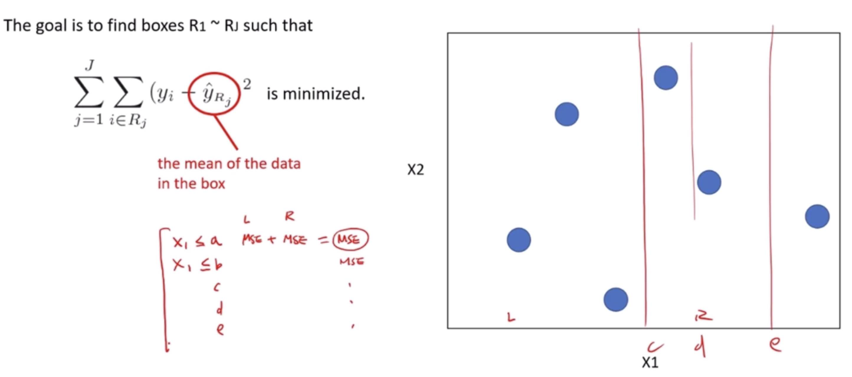
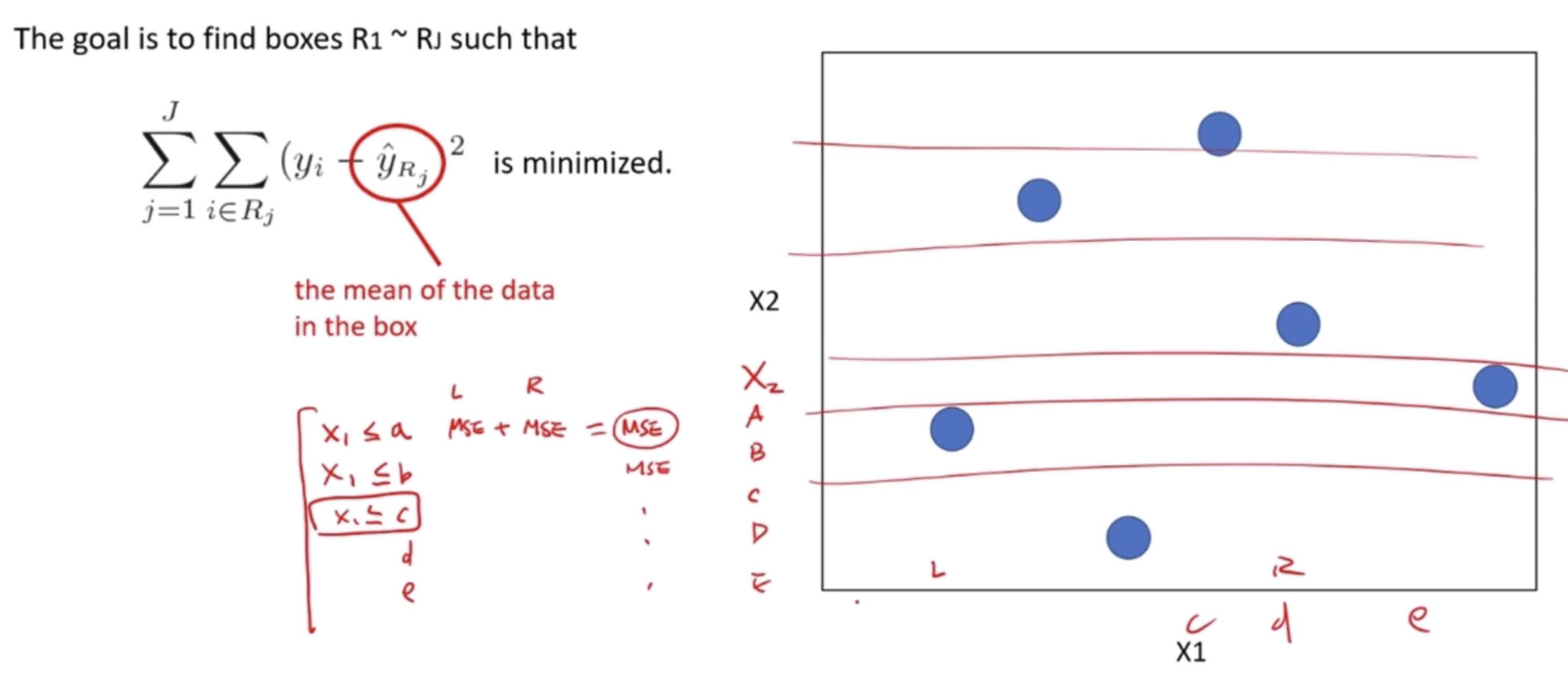
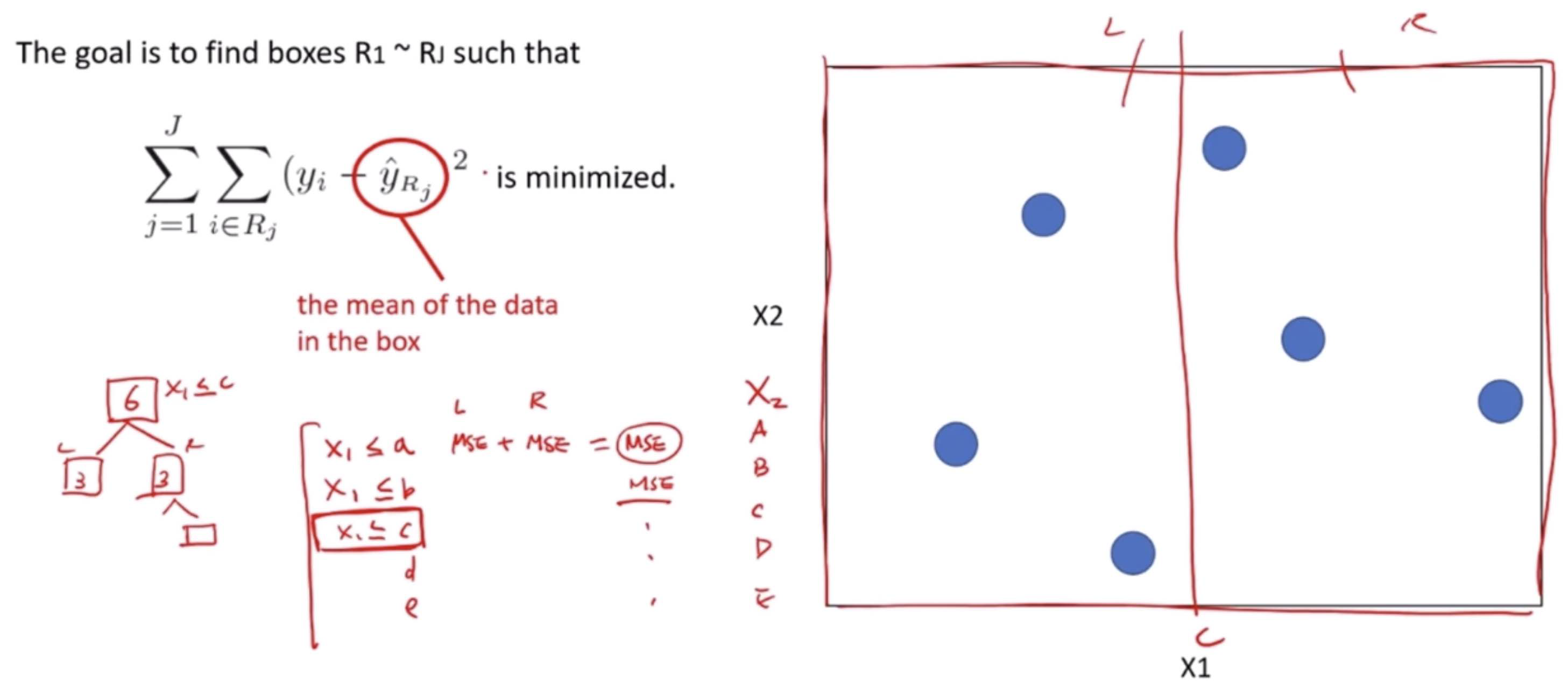
The Decision Tree Regressor uses the Mean Squared Error (MSE) as a measure to decide on the best split at each decision node. MSE is a popular metric used to evaluate the performance of a regression model, indicating the average squared difference between the observed actual outturns and the predictions made by the model. The goal of the regressor is to minimize the MSE at each step of building the tree.
How it Works Using MSE
Starting at the Root: The entire dataset is considered as the root.
Best Split Decision: To decide on a split, it calculates the MSE for every possible split in every feature and chooses the one that results in the lowest MSE. This split is the one that, if used to split the dataset into two groups, would result in the most similar responses within each group.
Recursion on Subsets: This process of finding the best split is then recursively applied to each resulting subset. The recursion is completed when the algorithm reaches a predetermined stopping criterion, such as a maximum depth of the tree or a minimum number of samples required to split a node further.
Prediction: For a prediction, the input features of a new data point are fed through the decision tree. The path followed by the data point through the tree leads to a leaf node. The average of the values in this leaf node is used as the prediction.
Example
Imagine we are using a dataset of houses, where our features include the number of bedrooms, the number of bathrooms, square footage, and the year built, and our target variable is the house price.
Root: Initially, the entire dataset is the root.
Best Split Calculation: The algorithm evaluates all features and their possible values to find the split that would result in subsets with the most similar house prices (lowest MSE). Suppose the best initial split divides the dataset into houses with less than 2 bathrooms and houses with 2 or more bathrooms.
Recursive Splitting: This process continues, with each subset being split on features and feature values that minimize the MSE within each resulting subset. For instance, within the subset of houses with less than 2 bathrooms, the next split might be on the number of bedrooms.
Stopping Criterion Reached: Eventually, when the stopping criteria are met (for example, a maximum depth of the tree), the splitting stops.
Making Predictions: To predict the price of a new house, we would input its features into the decision tree. The house would follow a path down the tree determined by its features until it reaches a leaf node. The prediction would be the average price of the houses in that leaf node.
This example simplifies the complexity involved in building a decision tree regressor but gives an outline of how MSE is used to create a model that can predict continuous outcomes like house prices.


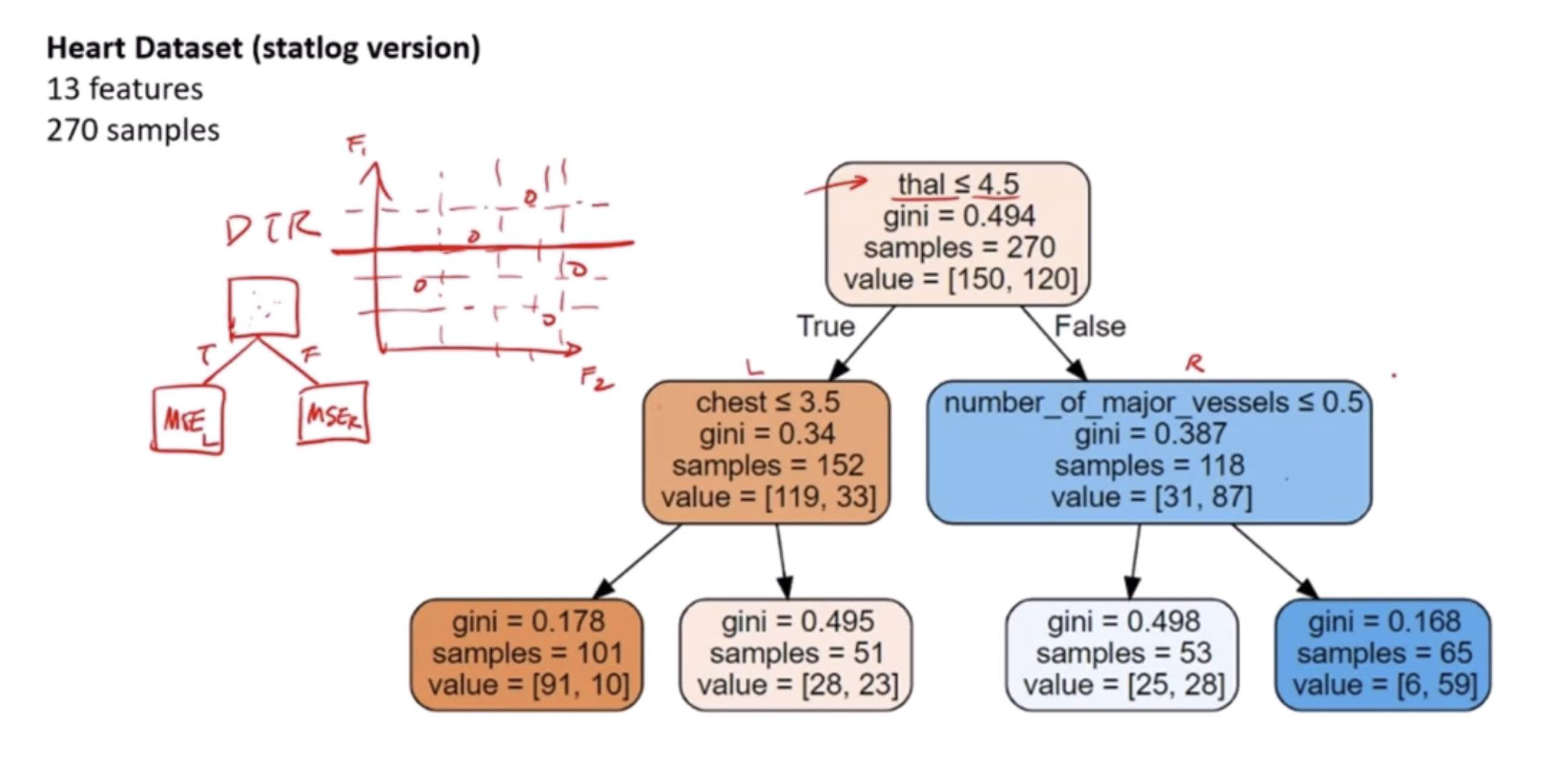
Decision Tree Classifier
Decision Tree Classifier is similar to Decision Tree Regressor, with the difference that it classifies the target variable.
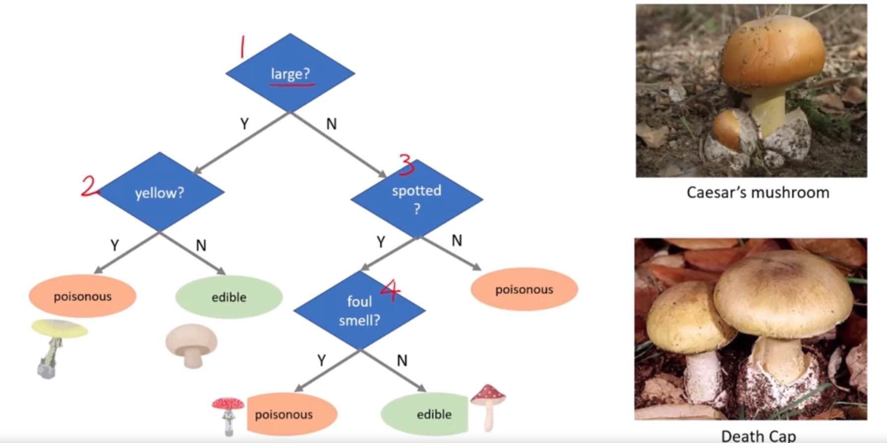
A Decision Tree Classifier is a flowchart-like structure in which each internal node represents a “test” on an attribute (e.g., “Is the animal you’re thinking of larger than a breadbox?”), each branch represents the outcome of the test, and each leaf node represents a class label (decision taken after computing all attributes). The paths from root to leaf represent classification rules.
How it works:
Starting at the root: Based on the data (features of animals in our analogy), the algorithm chooses the most significant feature to split the data into groups. This is usually done using measures like Gini impurity or information gain to determine which feature brings us closer to a decision.
Splitting: This process is repeated for each child node (e.g., if the first question splits the animals into “larger than a breadbox” and “not larger than a breadbox,” each of those groups is then split again based on another feature), creating the tree.
Stopping Criteria: The tree stops growing when it meets a stopping criterion, like when it can no longer reduce uncertainty or when it reaches a specified depth.
Decision Making: Once built, you can use the tree to classify new cases (predict the class of a new animal) by following the decisions in the tree based on the features of the new case.
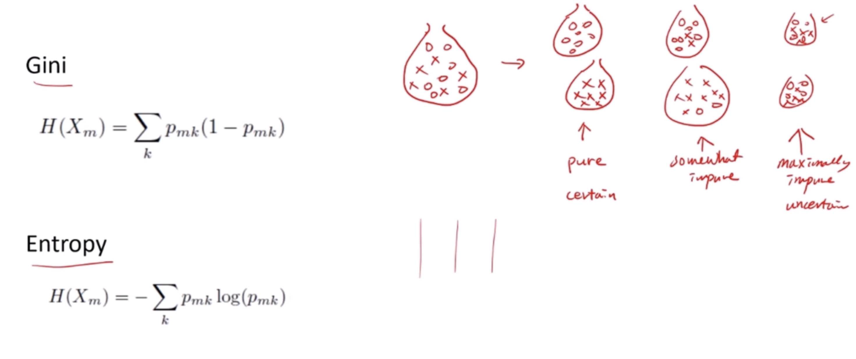
Gini Impurity: Simplified
The Gini impurity formula you’ve provided is a mathematical way to quantify how “pure” a set (usually a set of data points in a decision tree node) is. It tells us what the chance is that a randomly chosen element from the set is incorrectly labeled if it was randomly labeled according to the distribution of classes in the set. Let’s break it down:
\( H(X_m) \) is the Gini impurity of a set \( m \).
\( p_{mk} \) is the proportion (or probability) of class \( k \) in the set \( m \)
The formula sums up the product of the probability of each class with the probability of not being that class (which is \( 1 - p_{mk} \)). This product gives a measure of the probability of misclassification for each class. By summing over all classes, the Gini impurity considers the probability of misclassification regardless of what class we’re talking about.
Let’s go through a step-by-step example with a tangible dataset.
Example Dataset:
Imagine we have a small dataset of 10 animals, with two features: “Can Fly” (Yes or No) and “Has Fins” (Yes or No). We want to classify them into two classes: “Bird” or “Fish”.
Here are the animals:
4 are birds that can fly.
2 are birds that cannot fly (perhaps penguins).
3 are fish that have fins.
1 is a fish that does not have fins (maybe an eel).
Step 1: Calculate Class Proportions
We first need to calculate the proportions of each class in the set.
Birds: \( p_{bird} = \frac{4 + 2}{10} = \frac{6}{10} = 0.6 \)
Fish: \( p_{fish} = \frac{3 + 1}{10} = \frac{4}{10} = 0.4 \)
Step 2: Plug Proportions Into the Formula
Now we use the Gini formula.
Gini for birds: \( p_{bird} \times (1 - p_{bird}) = 0.6 \times (1 - 0.6) = 0.6 \times 0.4 = 0.24 \)
Gini for fish: \( p_{fish} \times (1 - p_{fish}) = 0.4 \times (1 - 0.4) = 0.4 \times 0.6 = 0.24 \)
Step 3: Sum the Gini for All Classes
The Gini impurity for the set is the sum of the Gini for all classes.
Total Gini impurity: \( H(X_m) = 0.24 + 0.24 = 0.48 \)
This Gini impurity value of 0.48 is relatively high, indicating that the set is quite mixed (if it were 0, the set would be perfectly pure).
Step 4: Interpretation
A Gini impurity of 0.48 means that if we pick a random animal from this dataset and then randomly assign a label based on the distribution of the classes (60% chance of being labeled as a bird and 40% as a fish), there’s a 48% chance of mislabeling the animal.
The goal in a decision tree is to create splits that result in subsets with lower Gini impurity scores compared to the parent node. A perfect split would be one that results in nodes with a Gini impurity of 0, meaning all elements in each node are from a single class.
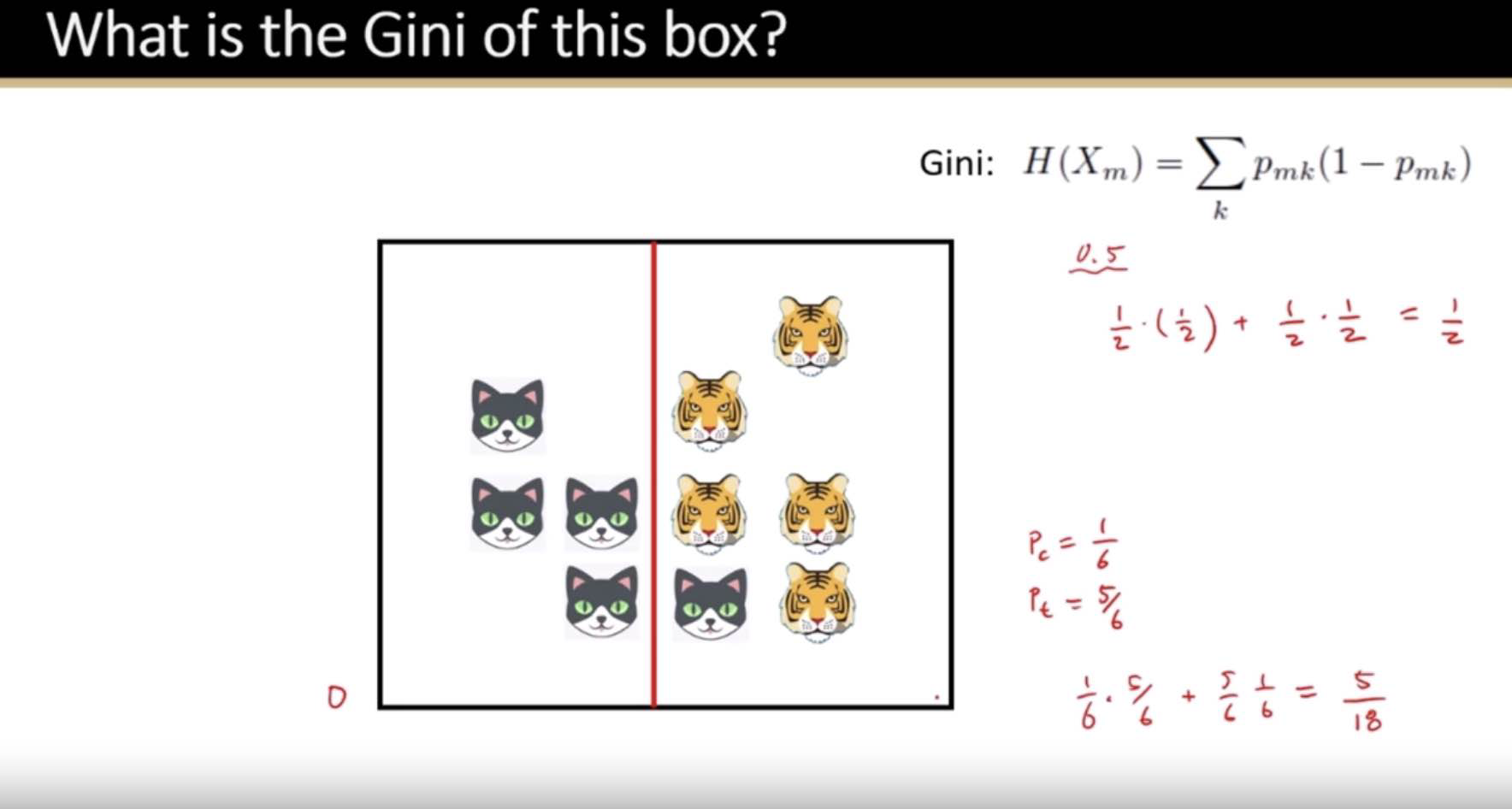
Gini Impurity = 1 - sum (probability of each class)^2
The best (lowest) Gini impurity is 0, where all elements belong to a single class (pure). The worst (highest) Gini impurity is 0.5 in a binary classification, where the dataset is evenly split between two classes (completely mixed).
Example:
Let’s say we have a dataset of 10 animals, 6 are fish and 4 are birds.
The probability of picking a fish randomly is 6/10, and the probability of picking a bird is 4/10.
Gini Impurity = 1 - ( (6/10)^2 + (4/10)^2 ) = 1 - ( 0.36 + 0.16 ) = 1 - 0.52 = 0.48
This Gini score tells us how often we would be wrong if we randomly assigned a label to an animal in this group based on the distribution of classes. A lower score is better, indicating less impurity.
We’ll apply the Gini impurity formula:
For the given probabilities of the two classes:
\( p_{\text{class1}} = 0.77777777777 \) \( p_{\text{class2}} = 0.22222222222 \)
The Gini impurity for each class is calculated as:
For class 1: \( H(X_{m1}) = p_{\text{class1}} (1 - p_{\text{class1}}) = 0.77777777777 \times (1 - 0.77777777777) \)
For class 2: \( H(X_{m2}) = p_{\text{class2}} (1 - p_{\text{class2}}) = 0.22222222222 \times (1 - 0.22222222222) \)
Adding the Gini impurity of both classes:
The Gini impurity for the binary classification with the given class probabilities is approximately 0.3457.
Ensemble Methods
Ensemble methods are techniques that combine multiple models to improve the robustness and accuracy of predictions. These methods work on the principle that a group of “weak learners” can come together to form a “strong learner.”
Bagging (Bootstrap Aggregating)
Bagging reduces variance and helps to avoid overfitting. It involves creating multiple versions of a predictor and using these to get an aggregated predictor. The steps are:
Randomly create “bootstrap” samples of the original dataset (with replacement).
Train a model on each of these samples.
Combine the models using the average (regression) or majority vote (classification).
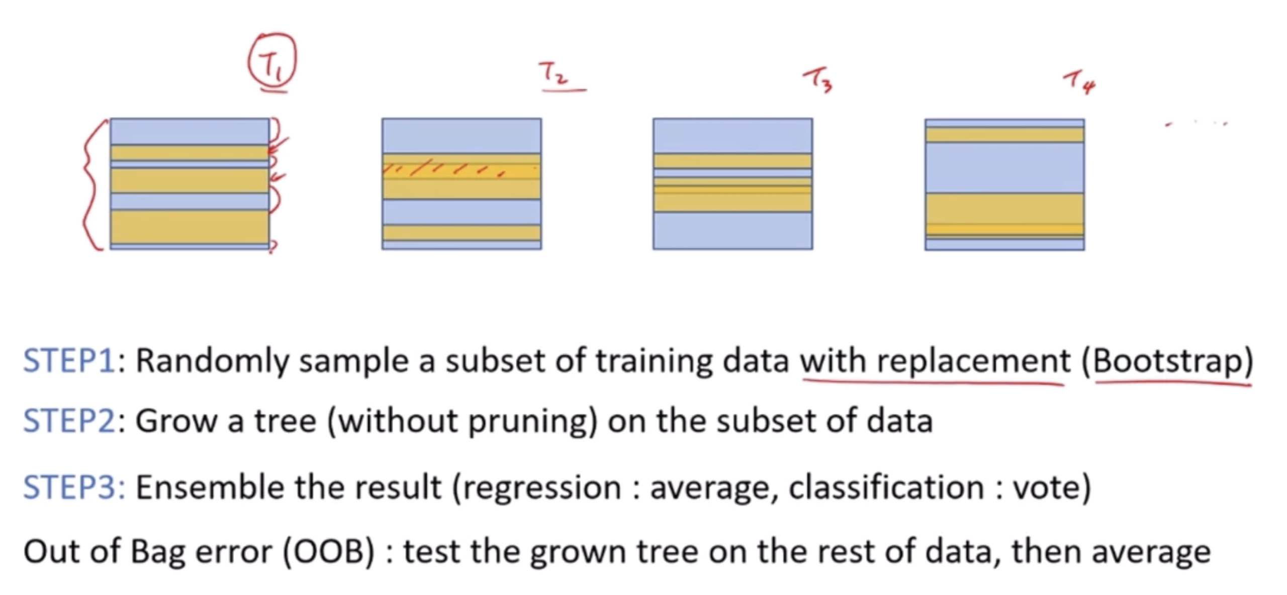
Example: Random Forest is a popular bagging ensemble of decision trees. Each tree is built on a bootstrap sample of the data, and the final prediction is averaged across all trees.


Boosting
Boosting focuses on converting weak learners into strong learners sequentially. Each model attempts to correct the errors made by the previous ones. The steps include:
Train a model on the entire dataset.
Build another model to correct the errors of the first model.
Continue adding models until a limit is reached or no further improvements can be made.
The final model makes predictions based on the weighted sum of the predictions of all models.

Examples: AdaBoost (Adaptive Boosting) and Gradient Boosting are well-known boosting methods. AdaBoost adjusts the weights of incorrectly classified instances so that subsequent classifiers focus more on difficult cases.
Advantages of Ensemble Methods
Improved Accuracy: Combining models often yields better results than any single model.
Reduced Overfitting: Especially with bagging and stacking, since they average out biases.
Increased Robustness: The ensemble’s prediction is less sensitive to noise and outliers.
Disadvantages of Ensemble Methods
Increased Complexity: More parameters to tune and a more complicated model to explain.
Higher Computational Cost: Training multiple models is computationally more expensive.
Risk of Overfitting with Boosting: Especially if the dataset is noisy.
Ensemble methods are widely used in various applications, from competitive machine learning competitions to practical business problems, because of their ability to improve prediction accuracy and model robustness.
Adaboost
The AdaBoost (Adaptive Boosting) algorithm is a powerful ensemble technique used to improve the performance of binary classifiers. It combines multiple weak learners (a learner that performs slightly better than random guessing) to create a strong classifier. Here’s a detailed breakdown of how AdaBoost works and the key formula involved:
How AdaBoost Works:
Initialization: Each observation in the dataset is initially given an equal weight. This signifies that at the start, every instance is equally important for the model.
Iterative Training:
Weak Learner Training: In each round, a weak learner is trained on the dataset. The goal of this learner is only to be slightly better than random guessing, regardless of its complexity.
Error Calculation: After training a weak learner, AdaBoost calculates the error rate of the learner. This error is weighted based on the weights of the observations. The error rate (\( \epsilon \)) is essentially the sum of the weights of the incorrectly classified observations divided by the sum of all weights.
Learner Weight Calculation: AdaBoost assigns a weight (\( \alpha \)) to the weak learner based on its accuracy. More accurate learners are given more weight. The weight is calculated using the formula: \( \alpha = \frac{1}{2} \ln\left(\frac{1 - \epsilon}{\epsilon}\right) \), where \( \ln \) is the natural logarithm.
Update Weights: The weights of the observations are updated so that the weights of the incorrectly classified observations are increased, and the weights of the correctly classified observations are decreased. This makes the algorithm focus more on the harder-to-classify instances in the next round.
Normalization: The updated weights are normalized so that their sum is 1.
Final Model:
After a specified number of rounds, or if perfect prediction is achieved, AdaBoost combines the weak learners into a final model. The final model makes predictions based on a weighted majority vote (or sum) of the weak learners’ predictions. Each weak learner’s vote is weighted by its \( \alpha \) value.
Key Formulae:
Error of a Weak Learner: \( \epsilon = \frac{\sum_{i=1}^{N} w_i \cdot \text{error}_i}{\sum_{i=1}^{N} w_i} \), where \( w_i \) is the weight of the \( i^{th} \) observation, and \( \text{error}_i \) is an indicator function that is 1 if the observation is misclassified and 0 otherwise.
Weight of a Weak Learner: \( \alpha = \frac{1}{2} \ln\left(\frac{1 - \epsilon}{\epsilon}\right) \).
Weight Update Rule: For each observation, the new weight (\( w_i' \)) is updated using the rule: \( w_i' = w_i \cdot e^{\alpha \cdot \text{error}_i} \), followed by a normalization step.
Conclusion:
AdaBoost is effective because it focuses on the observations that are hard to classify and gives more importance to the more accurate learners. This adaptiveness to the errors of the learners makes it a powerful algorithm for classification problems. The sequential process of adjusting weights puts more focus on instances that are hard to predict, leading to a highly accurate ensemble model.
Gradient Boosting
Gradient Boosting is a powerful machine learning algorithm that’s used for both regression and classification problems. It builds a model in a stage-wise fashion like AdaBoost, but it generalizes the boosting process by allowing optimization of an arbitrary differentiable loss function.
How Gradient Boosting Works:
Initialization: It begins with a simple model (often a decision tree), which could be just a prediction of the mean of the target values. This initial model serves as the base upon which further models (often called trees) are added.
Sequential Tree Building:
For each iteration, the algorithm first calculates the residuals or errors of the current model. In the context of regression, these are simply the differences between the predicted and actual values. In classification, the process is slightly more complex, involving the gradient of the loss function.
A new model (tree) is then trained to predict these residuals or gradients. Essentially, instead of directly predicting the target value or class, each new model aims to correct the mistakes of the combined ensemble of all previous models.
Once the new model is trained on the residuals, it is added to the ensemble. The idea is to take a step in the direction that minimizes the loss, akin to the gradient descent optimization algorithm, hence the name “Gradient Boosting.”
Loss Function Optimization:
Gradient Boosting involves the minimization of a loss function. The loss function quantifies how far off a prediction is from the actual result. The choice of loss function depends on the type of problem (regression, classification, etc.).
After each tree is added, the algorithm updates the predictions for each observation, effectively taking a step that reduces the loss (error).
Shrinkage (Learning Rate):
To prevent overfitting, Gradient Boosting introduces a learning rate (also known as “shrinkage”) that scales the contribution of each tree. A smaller learning rate requires more trees to model the data but generally results in a more robust model.
Example:
Imagine we’re trying to predict the price of houses based on features like size, location, and number of bedrooms. Our initial model might predict that each house costs $300,000, which is the average price of all houses in the training set.
First Iteration: We calculate the residuals (actual price - predicted price) for each house. Then, we train a decision tree to predict these residuals based on our features.
Update Predictions: We add this new tree to our model, adjusting our predictions for each house. Suppose this tree predicts that houses with 3 bedrooms are undervalued by $50,000. Our updated predictions for 3-bedroom houses would increase by this amount.
Repeat: We calculate new residuals based on our updated predictions and train a new tree to predict these residuals. This process repeats, with each new tree correcting the errors of the ensemble so far.
Final Model: After a specified number of iterations, or once our loss has been minimized to an acceptable level, we combine all the trees to make final predictions.
Conclusion:
Gradient Boosting is a versatile and powerful technique capable of handling both regression and classification problems. Its sequential nature, focusing on correcting its own errors, makes it highly effective, though it can be prone to overfitting if not properly regularized or if too many trees are used. The learning rate and the number of trees are crucial hyperparameters that need careful tuning to achieve the best performance.