PyTorch Neural Network Classification

For example, you might want to:

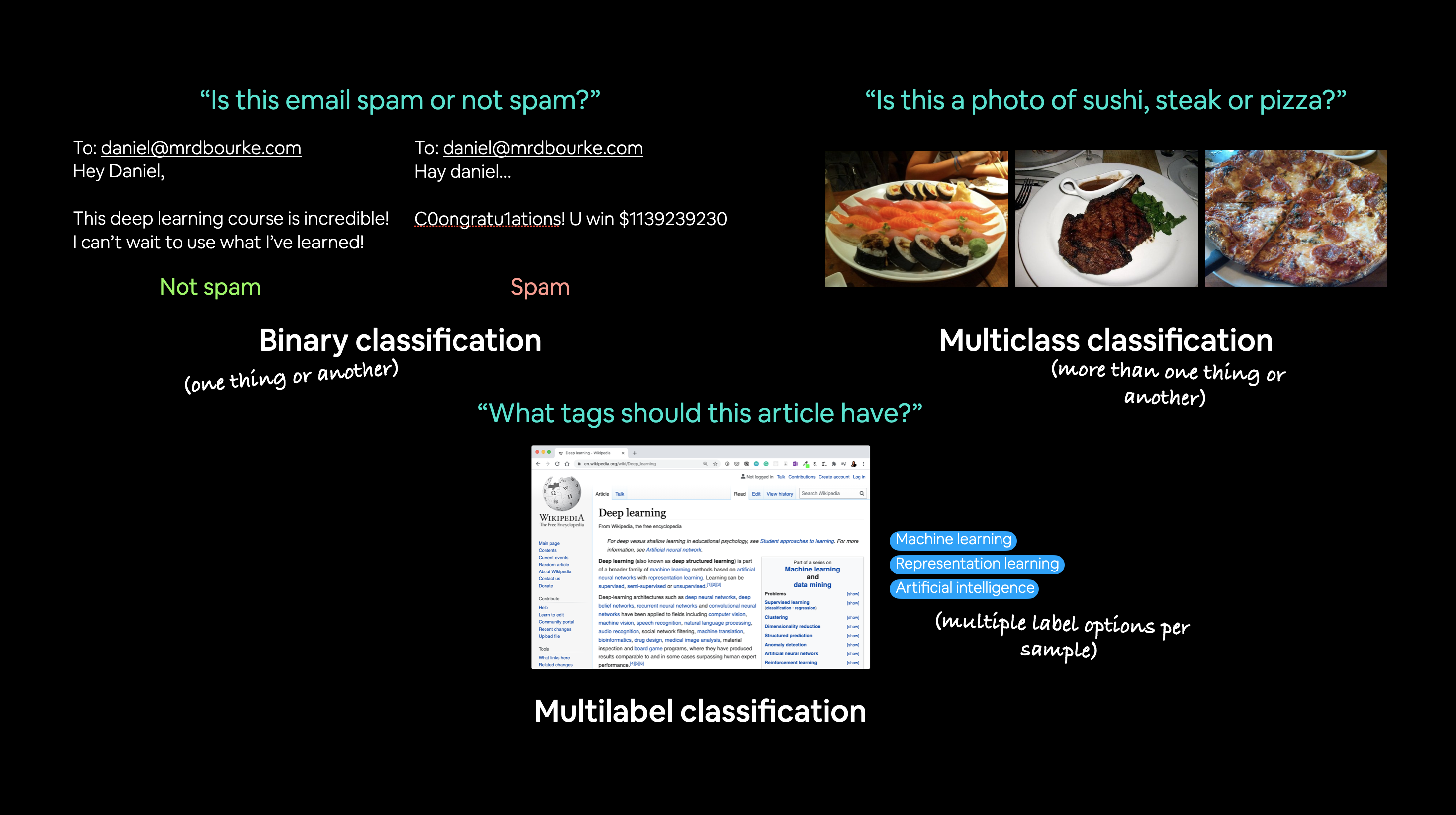
Problem type	What is it?	Example
Binary classification	Target can be one of two options, e.g. yes or no	Predict whether or not someone has heart disease based on their health parameters.
Multi-class classification	Target can be one of more than two options	Decide whether a photo of is of food, a person or a dog.
Multi-label classification	Target can be assigned more than one option	Predict what categories should be assigned to a Wikipedia article (e.g. mathematics, science & philosohpy).

In this notebook, we’re going to work through a couple of different classification problems with PyTorch.

In other words, taking a set of inputs and predicting what class those set of inputs belong to.

Architecture

Before we get into writing code, let’s look at the general architecture of a classification neural network.

Hyperparameter	Binary Classification	Multiclass classification
Input layer shape (in_features)	Same as number of features (e.g. 5 for age, sex, height, weight, smoking status in heart disease prediction)	Same as binary classification
Hidden layer(s)	Problem specific, minimum = 1, maximum = unlimited	Same as binary classification
Neurons per hidden layer	Problem specific, generally 10 to 512	Same as binary classification
Output layer shape (out_features)	1 (one class or the other)	1 per class (e.g. 3 for food, person or dog photo)
Hidden layer activation	Usually ReLU (rectified linear unit) but can be many others	Same as binary classification
Output activation	Sigmoid (torch.sigmoid in PyTorch)	Softmax (torch.softmax in PyTorch)
Loss function	Binary crossentropy (torch.nn.BCELoss in PyTorch)	Cross entropy (torch.nn.CrossEntropyLoss in PyTorch)
Optimizer	SGD (stochastic gradient descent), Adam (see torch.optim for more options)	Same as binary classification

Of course, this ingredient list of classification neural network components will vary depending on the problem you’re working on.

But it’s more than enough to get started.

We’re going to gets hands-on with this setup throughout this notebook.

Make classification data

We’ll use the make_circles() method from Scikit-Learn to generate two circles with different coloured dots.

import torch

torch.__version__

'2.2.2+cu121'

from sklearn.datasets import make_circles


# Make 1000 samples 
n_samples = 1000

# Create circles
X, y = make_circles(n_samples,
                    noise=0.03, # a little bit of noise to the dots
                    random_state=42) # keep random state so we get the same values

print(f"First 5 X features:\n{X[:5]}")
print(f"\nFirst 5 y labels:\n{y[:5]}")

First 5 X features:
[[ 0.75424625  0.23148074]
 [-0.75615888  0.15325888]
 [-0.81539193  0.17328203]
 [-0.39373073  0.69288277]
 [ 0.44220765 -0.89672343]]

First 5 y labels:
[1 1 1 1 0]

# Make DataFrame of circle data
import pandas as pd
circles = pd.DataFrame({"X1": X[:, 0],
    "X2": X[:, 1],
    "label": y
})
circles.head(10)

	X1	X2	label
0	0.754246	0.231481	1
1	-0.756159	0.153259	1
2	-0.815392	0.173282	1
3	-0.393731	0.692883	1
4	0.442208	-0.896723	0
5	-0.479646	0.676435	1
6	-0.013648	0.803349	1
7	0.771513	0.147760	1
8	-0.169322	-0.793456	1
9	-0.121486	1.021509	0

# Check different labels
circles.label.value_counts()

label
1    500
0    500
Name: count, dtype: int64

# Visualize with a plot
import matplotlib.pyplot as plt
plt.scatter(x=X[:, 0], 
            y=X[:, 1], 
            c=y, 
            cmap=plt.cm.RdYlBu);

Input and output shapes

One of the most common errors in deep learning is shape errors.

Mismatching the shapes of tensors and tensor operations with result in errors in your models.

We’re going to see plenty of these throughout the course.

And there’s no surefire way to making sure they won’t happen, they will.

What you can do instead is continaully familiarize yourself with the shape of the data you’re working with.

I like referring to it as input and output shapes.

Ask yourself:

“What shapes are my inputs and what shapes are my outputs?”

# Check the shapes of our features and labels
X.shape, y.shape

((1000, 2), (1000,))

# View the first example of features and labels
X_sample = X[0]
y_sample = y[0]
print(f"Values for one sample of X: {X_sample} and the same for y: {y_sample}")
print(f"Shapes for one sample of X: {X_sample.shape} and the same for y: {y_sample.shape}")

Values for one sample of X: [0.75424625 0.23148074] and the same for y: 1
Shapes for one sample of X: (2,) and the same for y: ()

X = torch.from_numpy(X).type(torch.float)
y = torch.from_numpy(y).type(torch.float)

# View the first five samples
X[:5], y[:5]

(tensor([[ 0.7542,  0.2315],
         [-0.7562,  0.1533],
         [-0.8154,  0.1733],
         [-0.3937,  0.6929],
         [ 0.4422, -0.8967]]),
 tensor([1., 1., 1., 1., 0.]))

# Split data into train and test sets
from sklearn.model_selection import train_test_split

X_train, X_test, y_train, y_test = train_test_split(X, 
                                                    y, 
                                                    test_size=0.2, # 20% test, 80% train
                                                    random_state=42) # make the random split reproducible

len(X_train), len(X_test), len(y_train), len(y_test)

(800, 200, 800, 200)

Building a model

We’ll break it down into a few parts.

Setting up device agnostic code (so our model can run on CPU or GPU if it’s available). Constructing a model by subclassing nn.Module. Defining a loss function and optimizer. Creating a training loop (this’ll be in the next section).

# Standard PyTorch imports
from torch import nn

# Make device agnostic code
device = "cuda" if torch.cuda.is_available() else "cpu"
device

'cpu'

How about we create a model?

We’ll want a model capable of handling our X data as inputs and producing something in the shape of our y data as ouputs.

In other words, given X (features) we want our model to predict y (label).

This setup where you have features and labels is referred to as supervised learning. Because your data is telling your model what the outputs should be given a certain input.

To create such a model it’ll need to handle the input and output shapes of X and y.

Remember how I said input and output shapes are important? Here we’ll see why.

Let’s create a model class that:

Subclasses nn.Module (almost all PyTorch models are subclasses of nn.Module). Creates 2 nn.Linear layers in the constructor capable of handling the input and output shapes of X and y. Defines a forward() method containing the forward pass computation of the model. Instantiates the model class and sends it to the target device.

# 1. Construct a model class that subclasses nn.Module
class CircleModelV0(nn.Module):
    def __init__(self):
        super().__init__()
        # 2. Create 2 nn.Linear layers capable of handling X and y input and output shapes
        self.layer_1 = nn.Linear(in_features=2, out_features=5) # takes in 2 features (X), produces 5 features
        self.layer_2 = nn.Linear(in_features=5, out_features=1) # takes in 5 features, produces 1 feature (y)
    
    # 3. Define a forward method containing the forward pass computation
    def forward(self, x):
        # Return the output of layer_2, a single feature, the same shape as y
        return self.layer_2(self.layer_1(x)) # computation goes through layer_1 first then the output of layer_1 goes through layer_2

# 4. Create an instance of the model and send it to target device
model_0 = CircleModelV0().to(device)
model_0

CircleModelV0(
  (layer_1): Linear(in_features=2, out_features=5, bias=True)
  (layer_2): Linear(in_features=5, out_features=1, bias=True)
)

self.layer_1 takes 2 input features in_features=2 and produces 5 output features out_features=5.

This is known as having 5 hidden units or neurons.

This layer turns the input data from having 2 features to 5 features.

Why do this?

This allows the model to learn patterns from 5 numbers rather than just 2 numbers, potentially leading to better outputs.

I say potentially because sometimes it doesn’t work.

The number of hidden units you can use in neural network layers is a hyperparameter (a value you can set yourself) and there’s no set in stone value you have to use.

Generally more is better but there’s also such a thing as too much. The amount you choose will depend on your model type and dataset you’re working with.

Since our dataset is small and simple, we’ll keep it small.

The only rule with hidden units is that the next layer, in our case, self.layer_2 has to take the same in_features as the previous layer out_features.

That’s why self.layer_2 has in_features=5, it takes the out_features=5 from self.layer_1 and performs a linear computation on them, turning them into out_features=1 (the same shape as y).

You can also do the same as above using nn.Sequential.

nn.Sequential performs a forward pass computation of the input data through the layers in the order they appear.

# Replicate CircleModelV0 with nn.Sequential
model_0 = nn.Sequential(
    nn.Linear(in_features=2, out_features=5),
    nn.Linear(in_features=5, out_features=1)
).to(device)

model_0

Sequential(
  (0): Linear(in_features=2, out_features=5, bias=True)
  (1): Linear(in_features=5, out_features=1, bias=True)
)

# Make predictions with the model
untrained_preds = model_0(X_test.to(device))
print(f"Length of predictions: {len(untrained_preds)}, Shape: {untrained_preds.shape}")
print(f"Length of test samples: {len(y_test)}, Shape: {y_test.shape}")
print(f"\nFirst 10 predictions:\n{untrained_preds[:10]}")
print(f"\nFirst 10 test labels:\n{y_test[:10]}")

Length of predictions: 200, Shape: torch.Size([200, 1])
Length of test samples: 200, Shape: torch.Size([200])

First 10 predictions:
tensor([[0.8633],
        [0.9981],
        [0.3884],
        [0.9983],
        [0.1955],
        [0.2793],
        [0.8117],
        [0.6429],
        [0.3972],
        [1.0050]], grad_fn=<SliceBackward0>)

First 10 test labels:
tensor([1., 0., 1., 0., 1., 1., 0., 0., 1., 0.])

Setup loss function and optimizer

But different problem types require different loss functions.

For example, for a regression problem (predicting a number) you might used mean absolute error (MAE) loss.

And for a binary classification problem (like ours), you’ll often use binary cross entropy as the loss function.

However, the same optimizer function can often be used across different problem spaces.

For example, the stochastic gradient descent optimizer (SGD, torch.optim.SGD()) can be used for a range of problems, so can too the Adam optimizer (torch.optim.Adam()).

Loss function/Optimizer	Problem type	PyTorch Code
Stochastic Gradient Descent (SGD) optimizer	Classification, regression, many others.	torch.optim.SGD()
Adam Optimizer	Classification, regression, many others.	torch.optim.Adam()
Binary cross entropy loss	Binary classification	torch.nn.BCELossWithLogits or torch.nn.BCELoss
Cross entropy loss	Mutli-class classification	torch.nn.CrossEntropyLoss
Mean absolute error (MAE) or L1 Loss	Regression	torch.nn.L1Loss
Mean squared error (MSE) or L2 Loss	Regression	torch.nn.MSELoss

Table of various loss functions and optimizers, there are more but these some common ones you’ll see.

Since we’re working with a binary classification problem, let’s use a binary cross entropy loss function.

Note: Recall a loss function is what measures how wrong your model predictions are, the higher the loss, the worse your model.

Also, PyTorch documentation often refers to loss functions as “loss criterion” or “criterion”, these are all different ways of describing the same thing.

PyTorch has two binary cross entropy implementations:

1. torch.nn.BCELoss() - Creates a loss function that measures the binary cross entropy between the target (label) and input (features).

2. torch.nn.BCEWithLogitsLoss() - This is the same as above except it has a sigmoid layer (nn.Sigmoid) built-in (we’ll see what this means soon).

Which one should you use?

The documentation for torch.nn.BCEWithLogitsLoss() states that it’s more numerically stable than using torch.nn.BCELoss() after a nn.Sigmoid layer.

So generally, implementation 2 is a better option. However for advanced usage, you may want to separate the combination of nn.Sigmoid and torch.nn.BCELoss() but that is beyond the scope of this notebook.

Knowing this, let’s create a loss function and an optimizer.

For the optimizer we’ll use torch.optim.SGD() to optimize the model parameters with learning rate 0.1.

Note: There’s a discussion on the PyTorch forums about the use of nn.BCELoss vs. nn.BCEWithLogitsLoss. It can be confusing at first but as with many things, it becomes easier with practice.

# Create a loss function
# loss_fn = nn.BCELoss() # BCELoss = no sigmoid built-in
loss_fn = nn.BCEWithLogitsLoss() # BCEWithLogitsLoss = sigmoid built-in

# Create an optimizer
optimizer = torch.optim.SGD(params=model_0.parameters(), 
                            lr=0.1)

# Now let's also create an evaluation metric.
# Calculate accuracy (a classification metric)
def accuracy_fn(y_true, y_pred):
    correct = torch.eq(y_true, y_pred).sum().item() # torch.eq() calculates where two tensors are equal
    acc = (correct / len(y_pred)) * 100 
    return acc

Train model

Okay, now we’ve got a loss function and optimizer ready to go, let’s train a model.

Going from raw model outputs to predicted labels (logits -> prediction probabilities -> prediction labels) Before we the training loop steps, let’s see what comes out of our model during the forward pass (the forward pass is defined by the forward() method).

To do so, let’s pass the model some data.

# View the frist 5 outputs of the forward pass on the test data
y_logits = model_0(X_test.to(device))[:5]
y_logits

tensor([[0.8633],
        [0.9981],
        [0.3884],
        [0.9983],
        [0.1955]], grad_fn=<SliceBackward0>)

Since our model hasn’t been trained, these outputs are basically random.

But what are they?

They’re the output of our forward() method.

Which implements two layers of nn.Linear() which internally calls the following equation:

\[ \mathbf{y} = x \cdot \mathbf{Weights}^T + \mathbf{bias} \]

The raw outputs (unmodified) of this equation (\(\mathbf{y}\)) and in turn, the raw outputs of our model are often referred to as logits.

That’s what our model is outputing above when it takes in the input data (\(x\) in the equation or X_test in the code), logits.

However, these numbers are hard to interpret.

We’d like some numbers that are comparable to our truth labels.

To get our model’s raw outputs (logits) into such a form, we can use the sigmoid activation function.

Let’s try it out.

# Use sigmoid on model logits
y_pred_probs = torch.sigmoid(y_logits)
y_pred_probs

tensor([[0.7033],
        [0.7307],
        [0.5959],
        [0.7307],
        [0.5487]], grad_fn=<SigmoidBackward0>)

They’re now in the form of prediction probabilities (I usually refer to these as y_pred_probs), in other words, the values are now how much the model thinks the data point belongs to one class or another.

In our case, since we’re dealing with binary classification, our ideal outputs are 0 or 1.

So these values can be viewed as a decision boundary.

The closer to 0, the more the model thinks the sample belongs to class 0, the closer to 1, the more the model thinks the sample belongs to class 1.

# Find the predicted labels (round the prediction probabilities)
y_preds = torch.round(y_pred_probs)

# In full
y_pred_labels = torch.round(torch.sigmoid(model_0(X_test.to(device))[:5]))

# Check for equality
print(torch.eq(y_preds.squeeze(), y_pred_labels.squeeze()))

# Get rid of extra dimension
y_preds,y_preds.squeeze()

tensor([True, True, True, True, True])

(tensor([[1.],
         [1.],
         [1.],
         [1.],
         [1.]], grad_fn=<RoundBackward0>),
 tensor([1., 1., 1., 1., 1.], grad_fn=<SqueezeBackward0>))

# Excellent! Now it looks like our model's predictions are in the same form as our truth labels (y_test)

y_test[:5]

tensor([1., 0., 1., 0., 1.])

Building a training and testing loop

Let’s start by training for 100 epochs and outputing the model’s progress every 10 epochs.

torch.manual_seed(42)

# Set the number of epochs
epochs = 100

# Put data to target device
X_train, y_train = X_train.to(device), y_train.to(device)
X_test, y_test = X_test.to(device), y_test.to(device)

# Build training and evaluation loop
for epoch in range(epochs):
    ### Training
    model_0.train()

    # 1. Forward pass (model outputs raw logits)
    y_logits = model_0(X_train).squeeze() # squeeze to remove extra `1` dimensions, this won't work unless model and data are on same device 
    y_pred = torch.round(torch.sigmoid(y_logits)) # turn logits -> pred probs -> pred labls
  
    # 2. Calculate loss/accuracy
    # loss = loss_fn(torch.sigmoid(y_logits), # Using nn.BCELoss you need torch.sigmoid()
    #                y_train) 
    loss = loss_fn(y_logits, # Using nn.BCEWithLogitsLoss works with raw logits
                   y_train) 
    acc = accuracy_fn(y_true=y_train, 
                      y_pred=y_pred) 

    # 3. Optimizer zero grad
    optimizer.zero_grad()

    # 4. Loss backwards
    loss.backward()

    # 5. Optimizer step
    optimizer.step()

    ### Testing
    model_0.eval()
    with torch.inference_mode():
        # 1. Forward pass
        test_logits = model_0(X_test).squeeze() 
        test_pred = torch.round(torch.sigmoid(test_logits))
        # 2. Caculate loss/accuracy
        test_loss = loss_fn(test_logits,
                            y_test)
        test_acc = accuracy_fn(y_true=y_test,
                               y_pred=test_pred)

    # Print out what's happening every 10 epochs
    if epoch % 10 == 0:
        print(f"Epoch: {epoch} | Loss: {loss:.5f}, Accuracy: {acc:.2f}% | Test loss: {test_loss:.5f}, Test acc: {test_acc:.2f}%")

Epoch: 0 | Loss: 0.73666, Accuracy: 50.00% | Test loss: 0.74926, Test acc: 50.00%
Epoch: 10 | Loss: 0.70883, Accuracy: 58.38% | Test loss: 0.71824, Test acc: 57.00%
Epoch: 20 | Loss: 0.69916, Accuracy: 54.37% | Test loss: 0.70636, Test acc: 49.50%
Epoch: 30 | Loss: 0.69570, Accuracy: 52.88% | Test loss: 0.70143, Test acc: 50.00%
Epoch: 40 | Loss: 0.69438, Accuracy: 52.12% | Test loss: 0.69913, Test acc: 49.00%
Epoch: 50 | Loss: 0.69381, Accuracy: 51.00% | Test loss: 0.69790, Test acc: 47.50%
Epoch: 60 | Loss: 0.69352, Accuracy: 51.12% | Test loss: 0.69714, Test acc: 48.50%
Epoch: 70 | Loss: 0.69335, Accuracy: 51.25% | Test loss: 0.69662, Test acc: 46.50%
Epoch: 80 | Loss: 0.69324, Accuracy: 51.12% | Test loss: 0.69625, Test acc: 46.50%
Epoch: 90 | Loss: 0.69317, Accuracy: 50.75% | Test loss: 0.69597, Test acc: 45.50%

The accuracy barely moves above 50% on each data split.

And because we’re working with a balanced binary classification problem, it means our model is performing as good as random guessing (with 500 samples of class 0 and class 1 a model predicting class 1 every single time would achieve 50% accuracy).

Evaluate the model

From the metrics it looks like our model is random guessing.

How could we investigate this further?

I’ve got an idea.

The data explorer’s motto!

“Visualize, visualize, visualize!”

Let’s make a plot of our model’s predictions, the data it’s trying to predict on and the decision boundary it’s creating for whether something is class 0 or class 1.

To do so, we’ll write some code to download and import the helper_functions.py script from the Learn PyTorch for Deep Learning repo.

It contains a helpful function called plot_decision_boundary() which creates a NumPy meshgrid to visually plot the different points where our model is predicting certain classes.

We’ll also import plot_predictions() which we wrote in notebook 01 to use later.

In machine learning terms, our model is underfitting, meaning it’s not learning predictive patterns from the data.

How could we improve this?

Improving a model

Let’s try to fix our model’s underfitting problem.

Focusing specifically on the model (not the data), there are a few ways we could do this.

Model improvement technique*	What does it do?
Add more layers	Each layer potentially increases the learning capabilities of the model with each layer being able to learn some kind of new pattern in the data, more layers is often referred to as making your neural network deeper.
Add more hidden units	Similar to the above, more hidden units per layer means a potential increase in learning capabilities of the model, more hidden units is often referred to as making your neural network wider.
Fitting for longer (more epochs)	Your model might learn more if it had more opportunities to look at the data.
Changing the activation functions	Some data just can’t be fit with only straight lines (like what we’ve seen), using non-linear activation functions can help with this (hint, hint).
Change the learning rate	Less model specific, but still related, the learning rate of the optimizer decides how much a model should change its parameters each step, too much and the model overcorrects, too little and it doesn’t learn enough.
Change the loss function	Again, less model specific but still important, different problems require different loss functions. For example, a binary cross entropy loss function won’t work with a multi-class classification problem.
Use transfer learning	Take a pretrained model from a problem domain similar to yours and adjust it to your own problem. We cover transfer learning in notebook 06.

Note: *because you can adjust all of these by hand, they’re referred to as hyperparameters.

And this is also where machine learning’s half art half science comes in, there’s no real way to know here what the best combination of values is for your project, best to follow the data scientist’s motto of “experiment, experiment, experiment”.

Let’s see what happens if we add an extra layer to our model, fit for longer (epochs=1000 instead of epochs=100) and increase the number of hidden units from 5 to 10.

We’ll follow the same steps we did above but with a few changed hyperparameters.

class CircleModelV1(nn.Module):
    def __init__(self):
        super().__init__()
        self.layer_1 = nn.Linear(in_features=2, out_features=10)
        self.layer_2 = nn.Linear(in_features=10, out_features=10) # extra layer
        self.layer_3 = nn.Linear(in_features=10, out_features=1)
        
    def forward(self, x): # note: always make sure forward is spelt correctly!
        # Creating a model like this is the same as below, though below
        # generally benefits from speedups where possible.
        # z = self.layer_1(x)
        # z = self.layer_2(z)
        # z = self.layer_3(z)
        # return z
        return self.layer_3(self.layer_2(self.layer_1(x)))

model_1 = CircleModelV1().to(device)
model_1

CircleModelV1(
  (layer_1): Linear(in_features=2, out_features=10, bias=True)
  (layer_2): Linear(in_features=10, out_features=10, bias=True)
  (layer_3): Linear(in_features=10, out_features=1, bias=True)
)

# loss_fn = nn.BCELoss() # Requires sigmoid on input
loss_fn = nn.BCEWithLogitsLoss() # Does not require sigmoid on input
optimizer = torch.optim.SGD(model_1.parameters(), lr=0.1)

# This time we'll train for longer (epochs=1000 vs epochs=100) and see if it improves our model.

torch.manual_seed(42)

epochs = 1000 # Train for longer

# Put data to target device
X_train, y_train = X_train.to(device), y_train.to(device)
X_test, y_test = X_test.to(device), y_test.to(device)

for epoch in range(epochs):
    ### Training
    # 1. Forward pass
    y_logits = model_1(X_train).squeeze()
    y_pred = torch.round(torch.sigmoid(y_logits)) # logits -> predicition probabilities -> prediction labels

    # 2. Calculate loss/accuracy
    loss = loss_fn(y_logits, y_train)
    acc = accuracy_fn(y_true=y_train, 
                      y_pred=y_pred)

    # 3. Optimizer zero grad
    optimizer.zero_grad()

    # 4. Loss backwards
    loss.backward()

    # 5. Optimizer step
    optimizer.step()

    ### Testing
    model_1.eval()
    with torch.inference_mode():
        # 1. Forward pass
        test_logits = model_1(X_test).squeeze() 
        test_pred = torch.round(torch.sigmoid(test_logits))
        # 2. Caculate loss/accuracy
        test_loss = loss_fn(test_logits,
                            y_test)
        test_acc = accuracy_fn(y_true=y_test,
                               y_pred=test_pred)

    # Print out what's happening every 10 epochs
    if epoch % 100 == 0:
        print(f"Epoch: {epoch} | Loss: {loss:.5f}, Accuracy: {acc:.2f}% | Test loss: {test_loss:.5f}, Test acc: {test_acc:.2f}%")

Epoch: 0 | Loss: 0.69396, Accuracy: 50.88% | Test loss: 0.69261, Test acc: 51.00%

Epoch: 100 | Loss: 0.69305, Accuracy: 50.38% | Test loss: 0.69379, Test acc: 48.00%

Epoch: 200 | Loss: 0.69299, Accuracy: 51.12% | Test loss: 0.69437, Test acc: 46.00%

Epoch: 300 | Loss: 0.69298, Accuracy: 51.62% | Test loss: 0.69458, Test acc: 45.00%

Epoch: 400 | Loss: 0.69298, Accuracy: 51.12% | Test loss: 0.69465, Test acc: 46.00%

Epoch: 500 | Loss: 0.69298, Accuracy: 51.00% | Test loss: 0.69467, Test acc: 46.00%

Epoch: 600 | Loss: 0.69298, Accuracy: 51.00% | Test loss: 0.69468, Test acc: 46.00%

Epoch: 700 | Loss: 0.69298, Accuracy: 51.00% | Test loss: 0.69468, Test acc: 46.00%

Epoch: 800 | Loss: 0.69298, Accuracy: 51.00% | Test loss: 0.69468, Test acc: 46.00%

Epoch: 900 | Loss: 0.69298, Accuracy: 51.00% | Test loss: 0.69468, Test acc: 46.00%

What? Our model trained for longer and with an extra layer but it still looks like it didn’t learn any patterns better than random guessing.

Our model is still drawing a straight line between the red and blue dots.

The missing piece: non-linearity

We’ve seen our model can draw straight (linear) lines, thanks to its linear layers.

But how about we give it the capacity to draw non-straight (non-linear) lines?

How?

Let’s find out.

# Make and plot data
import matplotlib.pyplot as plt
from sklearn.datasets import make_circles

n_samples = 1000

X, y = make_circles(n_samples=1000,
    noise=0.03,
    random_state=42,
)

plt.scatter(X[:, 0], X[:, 1], c=y, cmap=plt.cm.RdBu);

# Convert to tensors and split into train and test sets
import torch
from sklearn.model_selection import train_test_split

# Turn data into tensors
X = torch.from_numpy(X).type(torch.float)
y = torch.from_numpy(y).type(torch.float)

# Split into train and test sets
X_train, X_test, y_train, y_test = train_test_split(X, 
                                                    y, 
                                                    test_size=0.2,
                                                    random_state=42
)

X_train[:5], y_train[:5]

(tensor([[ 0.6579, -0.4651],
         [ 0.6319, -0.7347],
         [-1.0086, -0.1240],
         [-0.9666, -0.2256],
         [-0.1666,  0.7994]]),
 tensor([1., 0., 0., 0., 1.]))

Building a model with non-linearity

Now here comes the fun part.

What kind of pattern do you think you could draw with unlimited straight (linear) and non-straight (non-linear) lines?

I bet you could get pretty creative.

So far our neural networks have only been using linear (straight) line functions.

But the data we’ve been working with is non-linear (circles).

What do you think will happen when we introduce the capability for our model to use non-linear actviation functions?

Well let’s see.

PyTorch has a bunch of ready-made non-linear activation functions that do similiar but different things.

One of the most common and best performing is [ReLU](https://en.wikipedia.org/wiki/Rectifier_(neural_networks) (rectified linear-unit, torch.nn.ReLU()).

Rather than talk about it, let’s put it in our neural network between the hidden layers in the forward pass and see what happens.

# Build model with non-linear activation function
from torch import nn
class CircleModelV2(nn.Module):
    def __init__(self):
        super().__init__()
        self.layer_1 = nn.Linear(in_features=2, out_features=10)
        self.layer_2 = nn.Linear(in_features=10, out_features=10)
        self.layer_3 = nn.Linear(in_features=10, out_features=1)
        self.relu = nn.ReLU() # <- add in ReLU activation function
        # Can also put sigmoid in the model 
        # This would mean you don't need to use it on the predictions
        # self.sigmoid = nn.Sigmoid()

    def forward(self, x):
      # Intersperse the ReLU activation function between layers
       return self.layer_3(self.relu(self.layer_2(self.relu(self.layer_1(x)))))

model_3 = CircleModelV2().to(device)
print(model_3)

CircleModelV2(
  (layer_1): Linear(in_features=2, out_features=10, bias=True)
  (layer_2): Linear(in_features=10, out_features=10, bias=True)
  (layer_3): Linear(in_features=10, out_features=1, bias=True)
  (relu): ReLU()
)

# Setup loss and optimizer 
loss_fn = nn.BCEWithLogitsLoss()
optimizer = torch.optim.SGD(model_3.parameters(), lr=0.1)

# Fit the model
torch.manual_seed(42)
epochs = 1000

# Put all data on target device
X_train, y_train = X_train.to(device), y_train.to(device)
X_test, y_test = X_test.to(device), y_test.to(device)

for epoch in range(epochs):
    # 1. Forward pass
    y_logits = model_3(X_train).squeeze()
    y_pred = torch.round(torch.sigmoid(y_logits)) # logits -> prediction probabilities -> prediction labels
    
    # 2. Calculate loss and accuracy
    loss = loss_fn(y_logits, y_train) # BCEWithLogitsLoss calculates loss using logits
    acc = accuracy_fn(y_true=y_train, 
                      y_pred=y_pred)
    
    # 3. Optimizer zero grad
    optimizer.zero_grad()

    # 4. Loss backward
    loss.backward()

    # 5. Optimizer step
    optimizer.step()

    ### Testing
    model_3.eval()
    with torch.inference_mode():
      # 1. Forward pass
      test_logits = model_3(X_test).squeeze()
      test_pred = torch.round(torch.sigmoid(test_logits)) # logits -> prediction probabilities -> prediction labels
      # 2. Calcuate loss and accuracy
      test_loss = loss_fn(test_logits, y_test)
      test_acc = accuracy_fn(y_true=y_test,
                             y_pred=test_pred)

    # Print out what's happening
    if epoch % 100 == 0:
        print(f"Epoch: {epoch} | Loss: {loss:.5f}, Accuracy: {acc:.2f}% | Test Loss: {test_loss:.5f}, Test Accuracy: {test_acc:.2f}%")

Epoch: 0 | Loss: 0.69295, Accuracy: 50.00% | Test Loss: 0.69319, Test Accuracy: 50.00%
Epoch: 100 | Loss: 0.69115, Accuracy: 52.88% | Test Loss: 0.69102, Test Accuracy: 52.50%

Epoch: 200 | Loss: 0.68977, Accuracy: 53.37% | Test Loss: 0.68940, Test Accuracy: 55.00%
Epoch: 300 | Loss: 0.68795, Accuracy: 53.00% | Test Loss: 0.68723, Test Accuracy: 56.00%

Epoch: 400 | Loss: 0.68517, Accuracy: 52.75% | Test Loss: 0.68411, Test Accuracy: 56.50%
Epoch: 500 | Loss: 0.68102, Accuracy: 52.75% | Test Loss: 0.67941, Test Accuracy: 56.50%

Epoch: 600 | Loss: 0.67515, Accuracy: 54.50% | Test Loss: 0.67285, Test Accuracy: 56.00%
Epoch: 700 | Loss: 0.66659, Accuracy: 58.38% | Test Loss: 0.66322, Test Accuracy: 59.00%

Epoch: 800 | Loss: 0.65160, Accuracy: 64.00% | Test Loss: 0.64757, Test Accuracy: 67.50%
Epoch: 900 | Loss: 0.62362, Accuracy: 74.00% | Test Loss: 0.62145, Test Accuracy: 79.00%

Ho ho! That’s looking far better!

Evaluating a model trained with non-linear activation functions

Remember how our circle data is non-linear? Well, let’s see how our models predictions look now the model’s been trained with non-linear activation functions.

# Make predictions
model_3.eval()
with torch.inference_mode():
    y_preds = torch.round(torch.sigmoid(model_3(X_test))).squeeze()
y_preds[:10], y[:10] # want preds in same format as truth labels

(tensor([1., 0., 1., 0., 0., 1., 0., 0., 1., 0.]),
 tensor([1., 1., 1., 1., 0., 1., 1., 1., 1., 0.]))

Multi-class PyTorch model

We’ve covered a fair bit.

But now let’s put it all together using a multi-class classification problem.

Recall a binary classification problem deals with classifying something as one of two options (e.g. a photo as a cat photo or a dog photo) where as a multi-class classification problem deals with classifying something from a list of more than two options (e.g. classifying a photo as a cat a dog or a chicken).

Creating multi-class classification data

To begin a multi-class classification problem, let’s create some multi-class data.

To do so, we can leverage Scikit-Learn’s make_blobs() method.

This method will create however many classes (using the centers parameter) we want.

Specifically, let’s do the following:

Create some multi-class data with make_blobs(). Turn the data into tensors (the default of make_blobs() is to use NumPy arrays). Split the data into training and test sets using train_test_split(). Visualize the data.

# Import dependencies
import matplotlib.pyplot as plt
from sklearn.datasets import make_blobs
from sklearn.model_selection import train_test_split

# Set the hyperparameters for data creation
NUM_CLASSES = 4
NUM_FEATURES = 2
RANDOM_SEED = 42

# 1. Create multi-class data
X_blob, y_blob = make_blobs(n_samples=1000,
    n_features=NUM_FEATURES, # X features
    centers=NUM_CLASSES, # y labels 
    cluster_std=1.5, # give the clusters a little shake up (try changing this to 1.0, the default)
    random_state=RANDOM_SEED
)

# 2. Turn data into tensors
X_blob = torch.from_numpy(X_blob).type(torch.float)
y_blob = torch.from_numpy(y_blob).type(torch.LongTensor)
print(X_blob[:5], y_blob[:5])

# 3. Split into train and test sets
X_blob_train, X_blob_test, y_blob_train, y_blob_test = train_test_split(X_blob,
    y_blob,
    test_size=0.2,
    random_state=RANDOM_SEED
)

# 4. Plot data
plt.figure(figsize=(10, 7))
plt.scatter(X_blob[:, 0], X_blob[:, 1], c=y_blob, cmap=plt.cm.RdYlBu)

tensor([[-8.4134,  6.9352],
        [-5.7665, -6.4312],
        [-6.0421, -6.7661],
        [ 3.9508,  0.6984],
        [ 4.2505, -0.2815]]) tensor([3, 2, 2, 1, 1])

<matplotlib.collections.PathCollection at 0x7efeaa2a4150>

Multi-class classification model

We’ve created a few models in PyTorch so far.

You might also be starting to get an idea of how flexible neural networks are.

How about we build one similar to model_3 but this still capable of handling multi-class data?

To do so, let’s create a subclass of nn.Module that takes in three hyperparameters:

• input_features - the number of X features coming into the model.

• output_features - the ideal numbers of output features we’d like (this will be equivalent to NUM_CLASSES or the number of classes in your multi-class classification problem).

• hidden_units - the number of hidden neurons we’d like each hidden layer to use.

• Since we’re putting things together, let’s setup some device agnostic code (we don’t have to do this again in the same notebook, it’s only a reminder).

Then we’ll create the model class using the hyperparameters above.

# Build model
class BlobModel(nn.Module):
    def __init__(self, input_features, output_features, hidden_units=8):
        """Initializes all required hyperparameters for a multi-class classification model.

        Args:
            input_features (int): Number of input features to the model.
            out_features (int): Number of output features of the model
              (how many classes there are).
            hidden_units (int): Number of hidden units between layers, default 8.
        """
        super().__init__()
        self.linear_layer_stack = nn.Sequential(
            nn.Linear(in_features=input_features, out_features=hidden_units),
            # nn.ReLU(), # <- does our dataset require non-linear layers? (try uncommenting and see if the results change)
            nn.Linear(in_features=hidden_units, out_features=hidden_units),
            # nn.ReLU(), # <- does our dataset require non-linear layers? (try uncommenting and see if the results change)
            nn.Linear(in_features=hidden_units, out_features=output_features), # how many classes are there?
        )
    
    def forward(self, x):
        return self.linear_layer_stack(x)

# Create an instance of BlobModel and send it to the target device
model_4 = BlobModel(input_features=NUM_FEATURES, 
                    output_features=NUM_CLASSES, 
                    hidden_units=8).to(device)
model_4

BlobModel(
  (linear_layer_stack): Sequential(
    (0): Linear(in_features=2, out_features=8, bias=True)
    (1): Linear(in_features=8, out_features=8, bias=True)
    (2): Linear(in_features=8, out_features=4, bias=True)
  )
)

loss function and optimizer

Since we’re working on a multi-class classification problem, we’ll use the nn.CrossEntropyLoss() method as our loss function.

And we’ll stick with using SGD with a learning rate of 0.1 for optimizing our model_4 parameters.

# Create loss and optimizer
loss_fn = nn.CrossEntropyLoss()
optimizer = torch.optim.SGD(model_4.parameters(), 
                            lr=0.1) # exercise: try changing the learning rate here and seeing what happens to the model's performance

Getting prediction probabilities

Alright, we’ve got a loss function and optimizer ready, and we’re ready to train our model but before we do let’s do a single forward pass with our model to see if it works.

# Testing the input features calculation

w_ = torch.rand(3, 2)
b_ = torch.rand(3)

d = nn.Linear(in_features=2, out_features=3)(X_blob_train[:5])
formula = torch.matmul(X_blob_train[:5], w_.T) + b_
formula1 = X_blob_train[:5] @ w_.T + b_

d , w_ , b_ , formula, formula1, X_blob_train[:5], w_.T , X_blob_train[:5].shape, w_.T.shape

(tensor([[-0.6177, -2.3760,  1.3912],
         [ 7.0950,  0.8435,  2.5291],
         [ 0.7714,  6.1724, -5.1197],
         [ 1.7382,  4.3139, -3.0706],
         [ 6.2979,  1.4964,  1.5808]], grad_fn=<AddmmBackward0>),
 tensor([[0.0766, 0.8460],
         [0.3624, 0.3083],
         [0.0850, 0.0029]]),
 tensor([0.6431, 0.3908, 0.6947]),
 tensor([[ 3.8275,  3.2374,  1.1326],
         [ 8.5012,  2.3767,  0.4995],
         [-7.6581, -5.4860, -0.0560],
         [-3.5728, -3.1615,  0.1697],
         [ 6.4933,  1.4058,  0.4320]]),
 tensor([[ 3.8275,  3.2374,  1.1326],
         [ 8.5012,  2.3767,  0.4995],
         [-7.6581, -5.4860, -0.0560],
         [-3.5728, -3.1615,  0.1697],
         [ 6.4933,  1.4058,  0.4320]]),
 tensor([[ 5.0405,  3.3076],
         [-2.6249,  9.5260],
         [-8.5240, -9.0402],
         [-6.0262, -4.4375],
         [-3.3397,  7.2175]]),
 tensor([[0.0766, 0.3624, 0.0850],
         [0.8460, 0.3083, 0.0029]]),
 torch.Size([5, 2]),
 torch.Size([2, 3]))

# Perform a single forward pass on the data (we'll need to put it to the target device for it to work)
model_4(X_blob_train.to(device))[:5]

tensor([[-1.2711, -0.6494, -1.4740, -0.7044],
        [ 0.2210, -1.5439,  0.0420,  1.1531],
        [ 2.8698,  0.9143,  3.3169,  1.4027],
        [ 1.9576,  0.3125,  2.2244,  1.1324],
        [ 0.5458, -1.2381,  0.4441,  1.1804]], grad_fn=<SliceBackward0>)

# How many elements in a single prediction sample?
model_4(X_blob_train.to(device))[0].shape, NUM_CLASSES 

(torch.Size([4]), 4)

Wonderful, our model is predicting one value for each class that we have.

Do you remember what the raw outputs of our model are called?

Hint: it rhymes with “frog splits” (no animals were harmed in the creation of these materials).

If you guessed logits, you’d be correct.

So right now our model is outputing logits but what if we wanted to figure out exactly which label is was giving the sample?

As in, how do we go from logits -> prediction probabilities -> prediction labels just like we did with the binary classification problem?

That’s where the softmax activation function comes into play.

The softmax function calculates the probability of each prediction class being the actual predicted class compared to all other possible classes.

If this doesn’t make sense, let’s see in code.

# Make prediction logits with model
y_logits = model_4(X_blob_test.to(device))

# Perform softmax calculation on logits across dimension 1 to get prediction probabilities
y_pred_probs = torch.softmax(y_logits, dim=1) 
print(y_logits[:5])
print(y_pred_probs[:5])

tensor([[-1.2549, -0.8112, -1.4795, -0.5696],
        [ 1.7168, -1.2270,  1.7367,  2.1010],
        [ 2.2400,  0.7714,  2.6020,  1.0107],
        [-0.7993, -0.3723, -0.9138, -0.5388],
        [-0.4332, -1.6117, -0.6891,  0.6852]], grad_fn=<SliceBackward0>)
tensor([[0.1872, 0.2918, 0.1495, 0.3715],
        [0.2824, 0.0149, 0.2881, 0.4147],
        [0.3380, 0.0778, 0.4854, 0.0989],
        [0.2118, 0.3246, 0.1889, 0.2748],
        [0.1945, 0.0598, 0.1506, 0.5951]], grad_fn=<SliceBackward0>)

Hmm, what’s happened here?

It may still look like the outputs of the softmax function are jumbled numbers (and they are, since our model hasn’t been trained and is predicting using random patterns) but there’s a very specific thing different about each sample.

After passing the logits through the softmax function, each individual sample now adds to 1 (or very close to).

Let’s check.

# Sum the first sample output of the softmax activation function 
torch.sum(y_pred_probs[0])

tensor(1., grad_fn=<SumBackward0>)

These prediction probablities are essentially saying how much the model thinks the target X sample (the input) maps to each class.

Since there’s one value for each class in y_pred_probs, the index of the highest value is the class the model thinks the specific data sample most belongs to.

We can check which index has the highest value using torch.argmax().

# Which class does the model think is *most* likely at the index 0 sample?
print(y_pred_probs[0])
print(torch.argmax(y_pred_probs[0]))

tensor([0.1872, 0.2918, 0.1495, 0.3715], grad_fn=<SelectBackward0>)
tensor(3)

You can see the output of torch.argmax() returns 3, so for the features (X) of the sample at index 0, the model is predicting that the most likely class value (y) is 3.

Of course, right now this is just random guessing so it’s got a 25% chance of being right (since there’s four classes). But we can improve those chances by training the model.

Note: To summarize the above, a model’s raw output is referred to as logits.

For a multi-class classification problem, to turn the logits into prediction probabilities, you use the softmax activation function (torch.softmax).

The index of the value with the highest prediction probability is the class number the model thinks is most likely given the input features for that sample (although this is a prediction, it doesn’t mean it will be correct).

Creating a training and testing loop

Alright, now we’ve got all of the preparation steps out of the way, let’s write a training and testing loop to improve and evaluation our model.

We’ve done many of these steps before so much of this will be practice.

The only difference is that we’ll be adjusting the steps to turn the model outputs (logits) to prediction probabilities (using the softmax activation function) and then to prediction labels (by taking the argmax of the output of the softmax activation function).

Let’s train the model for epochs=100 and evaluate it every 10 epochs.

# Fit the model
torch.manual_seed(42)

# Set number of epochs
epochs = 100

# Put data to target device
X_blob_train, y_blob_train = X_blob_train.to(device), y_blob_train.to(device)
X_blob_test, y_blob_test = X_blob_test.to(device), y_blob_test.to(device)

for epoch in range(epochs):
    ### Training
    model_4.train()

    # 1. Forward pass
    y_logits = model_4(X_blob_train) # model outputs raw logits 
    y_pred = torch.softmax(y_logits, dim=1).argmax(dim=1) # go from logits -> prediction probabilities -> prediction labels
    # print(y_logits)
    # 2. Calculate loss and accuracy
    loss = loss_fn(y_logits, y_blob_train) 
    acc = accuracy_fn(y_true=y_blob_train,
                      y_pred=y_pred)

    # 3. Optimizer zero grad
    optimizer.zero_grad()

    # 4. Loss backwards
    loss.backward()

    # 5. Optimizer step
    optimizer.step()

    ### Testing
    model_4.eval()
    with torch.inference_mode():
      # 1. Forward pass
      test_logits = model_4(X_blob_test)
      test_pred = torch.softmax(test_logits, dim=1).argmax(dim=1)
      # 2. Calculate test loss and accuracy
      test_loss = loss_fn(test_logits, y_blob_test)
      test_acc = accuracy_fn(y_true=y_blob_test,
                             y_pred=test_pred)

    # Print out what's happening
    if epoch % 10 == 0:
        print(f"Epoch: {epoch} | Loss: {loss:.5f}, Acc: {acc:.2f}% | Test Loss: {test_loss:.5f}, Test Acc: {test_acc:.2f}%") 

Epoch: 0 | Loss: 1.04324, Acc: 65.50% | Test Loss: 0.57861, Test Acc: 95.50%
Epoch: 10 | Loss: 0.14398, Acc: 99.12% | Test Loss: 0.13037, Test Acc: 99.00%
Epoch: 20 | Loss: 0.08062, Acc: 99.12% | Test Loss: 0.07216, Test Acc: 99.50%
Epoch: 30 | Loss: 0.05924, Acc: 99.12% | Test Loss: 0.05133, Test Acc: 99.50%
Epoch: 40 | Loss: 0.04892, Acc: 99.00% | Test Loss: 0.04098, Test Acc: 99.50%
Epoch: 50 | Loss: 0.04295, Acc: 99.00% | Test Loss: 0.03486, Test Acc: 99.50%
Epoch: 60 | Loss: 0.03910, Acc: 99.00% | Test Loss: 0.03083, Test Acc: 99.50%
Epoch: 70 | Loss: 0.03643, Acc: 99.00% | Test Loss: 0.02799, Test Acc: 99.50%
Epoch: 80 | Loss: 0.03448, Acc: 99.00% | Test Loss: 0.02587, Test Acc: 99.50%
Epoch: 90 | Loss: 0.03300, Acc: 99.12% | Test Loss: 0.02423, Test Acc: 99.50%

evaluating predictions

It looks like our trained model is performaning pretty well.

But to make sure of this, let’s make some predictions and visualize them.

# Make predictions
model_4.eval()
with torch.inference_mode():
    y_logits = model_4(X_blob_test)

# View the first 10 predictions
y_logits[:10]

tensor([[  4.3377,  10.3539, -14.8948,  -9.7642],
        [  5.0142, -12.0371,   3.3860,  10.6699],
        [ -5.5885, -13.3448,  20.9894,  12.7711],
        [  1.8400,   7.5599,  -8.6016,  -6.9942],
        [  8.0727,   3.2906, -14.5998,  -3.6186],
        [  5.5844, -14.9521,   5.0168,  13.2891],
        [ -5.9739, -10.1913,  18.8655,   9.9179],
        [  7.0755,  -0.7601,  -9.5531,   0.1736],
        [ -5.5919, -18.5990,  25.5310,  17.5799],
        [  7.3142,   0.7197, -11.2017,  -1.2011]])

# Turn predicted logits in prediction probabilities
y_pred_probs = torch.softmax(y_logits, dim=1)

# Turn prediction probabilities into prediction labels
y_preds = y_pred_probs.argmax(dim=1)

# Compare first 10 model preds and test labels
print(f"Predictions: {y_preds[:10]}\nLabels: {y_blob_test[:10]}")
print(f"Test accuracy: {accuracy_fn(y_true=y_blob_test, y_pred=y_preds)}%")

Predictions: tensor([1, 3, 2, 1, 0, 3, 2, 0, 2, 0])
Labels: tensor([1, 3, 2, 1, 0, 3, 2, 0, 2, 0])
Test accuracy: 99.5%