Hypothesis Testing

Statistical inference is the process of learning about characteristics of a population based on what is observed in a relatively small sample from that population. A sample will never give us the entire picture though, and we are bound to make incorrect decisions from time to time.

We will learn how to derive and interpret appropriate tests to manage this error and how to evaluate when one test is better than another. we will learn how to construct and perform principled hypothesis tests for a wide range of problems and applications when they are not.

What is Hypothesis

Hypothesis testing is an act in statistics whereby an analyst tests an assumption regarding a population parameter.
Hypothesis testing is a formal procedure for investigating our ideas about the world using statistics. It is most often used by scientists to test specific predictions, called hypotheses, that arise from theories.

Note

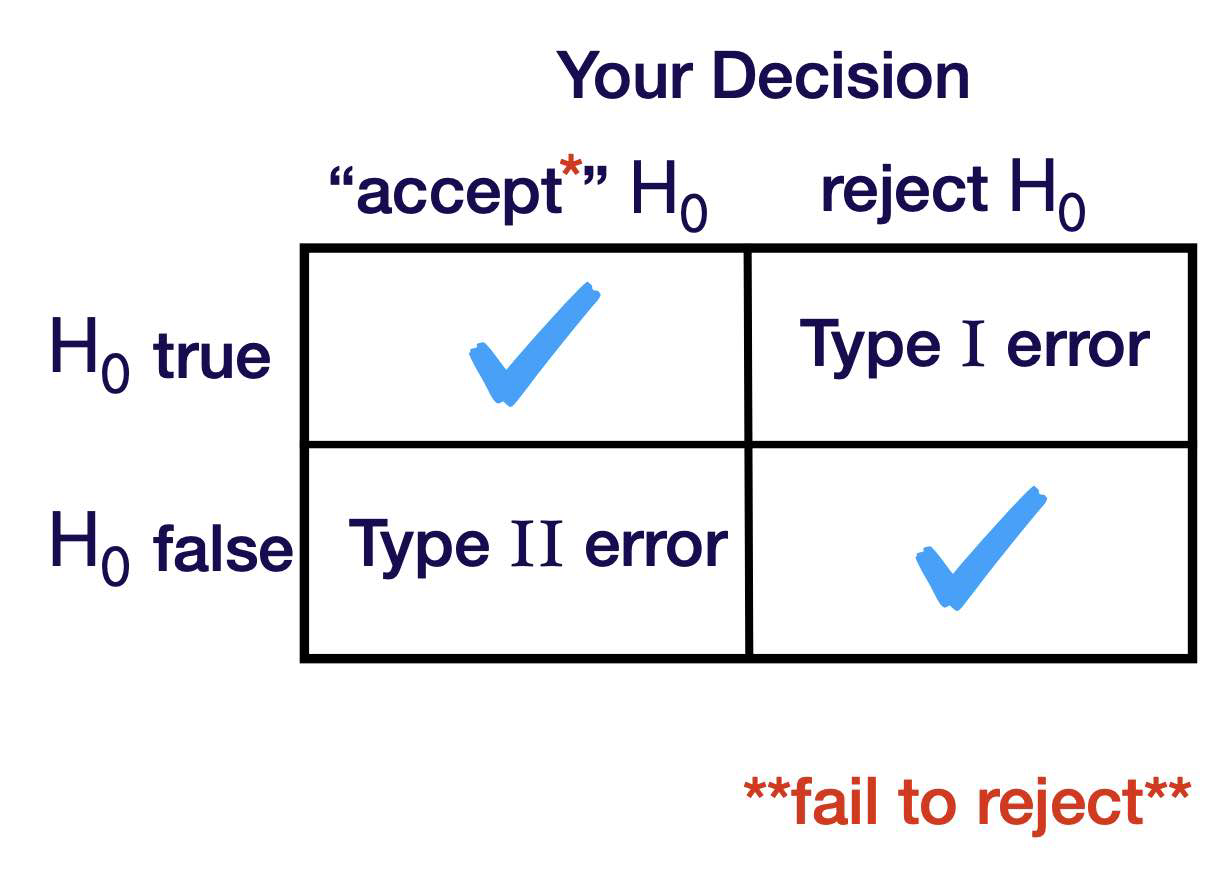
Due to random samples and randomness in the problem, we can different errors in our hypothesis testing. These errors are called Type I and Type II errors.

Type of hypothesis testing

Let $X_1, X_2, \ldots, X_n$ be a random sample from the normal distribution with mean $\mu$ and variance $\sigma^2$

import torch
import matplotlib.pyplot as plt
import seaborn as sns
from scipy.stats import norm


sns.set_theme(style="darkgrid")
sample = torch.normal(mean = 0, std = 1, size=(1,1000))

sns.displot(sample[0], kde=True, stat = 'density',)
plt.axvline(torch.mean(sample[0]), color='red', label='mean')
plt.show()

/home/docs/checkouts/readthedocs.org/user_builds/ml-math/envs/latest/lib/python3.10/site-packages/seaborn/_oldcore.py:1498: FutureWarning: is_categorical_dtype is deprecated and will be removed in a future version. Use isinstance(dtype, CategoricalDtype) instead
  if pd.api.types.is_categorical_dtype(vector):

/home/docs/checkouts/readthedocs.org/user_builds/ml-math/envs/latest/lib/python3.10/site-packages/seaborn/_oldcore.py:1119: FutureWarning: use_inf_as_na option is deprecated and will be removed in a future version. Convert inf values to NaN before operating instead.
  with pd.option_context('mode.use_inf_as_na', True):
/home/docs/checkouts/readthedocs.org/user_builds/ml-math/envs/latest/lib/python3.10/site-packages/seaborn/axisgrid.py:118: UserWarning: The figure layout has changed to tight
  self._figure.tight_layout(*args, **kwargs)

../_images/eff842a0f5a04f6697a4bfb01cf18c7ac0ce07d51d4591eb53261240ad29c39e.png

Example of random sample after it is observed:

\[ 2.73,1.14,3.98,2.15,5,85,1.97,2.54,2.03 \]

Based on what you are seeing, do you believe that the true population mean $\mu$ is

\[\begin{split} \mu<=3 \text{ or } \mu>3 \\ \text { The sample mean is } \overline{\mathrm{x}}=2.799 \end{split}\]

This is below 3 , but can we say that $\mu<3$ ?

This seems awfully dependent on the random sample we happened to get! Let’s try to work with the most generic random sample of size 8:

\[ X_1, X_2, X_3, X_4, X_5, X_6, X_7, X_8 \]

Let $\mathrm{X}_1, \mathrm{X}_2, \ldots, \mathrm{X}_{\mathrm{n}}$ be a random sample of size $\mathrm{n}$ from the $\mathrm{N}\left(\mu, \sigma^2\right)$ distribution.

\[ \mathrm{X}_1, \mathrm{X}_2, \ldots, \mathrm{X}_{\mathrm{n}} \stackrel{\text { iid }}{\sim} \mathrm{N}\left(\mu, \sigma^2\right) \]

The Sample mean is

\[ \bar{x}=\frac{1}{n} \sum_{i=11}^n X_i \]

We’re going to tend to think that $\mu<3$ when $\bar{X}$ is “significantly” smaller than 3.
We’re going to tend to think that $\mu>3$ when $\bar{X}$ is “significantly” larger than 3.
We’re never going to observe $\bar{X}=3$, but we may be able to be convinced that $\mu=3$ if $\bar{X}$ is not too far away.

How do we formalize this stuff, We use hypothesis testing

Notation

$\mathrm{H}_0: \mu \leq 3$ <- Null hypothesis
$\mathrm{H}_1: \mu>3 \quad$ Alternate hypothesis

Null hypothesis

The null hypothesis is a hypothesis that is assumed to be true. We denote it with an $H_0$.

Alternate hypothesis

The alternate hypothesis is what we are out to show. The alternative hypothesis is a hypothesis that we are looking for evidence for or out to show. We denote it with an $H_1$.

Note

Some people use the notation $H_a$ here

Conclusion is either:
Reject $\mathrm{H}_0 \quad$ OR $\quad$ Fail to Reject $\mathrm{H}_0$

simple hypothesis

A simple hypothesis is one that completely specifies the distribution. Do you know the exact distribution.

composite hypothesis

You don’t know the exact distribution.
Means you know the distribution is normal but you don’t know the mean and variance.

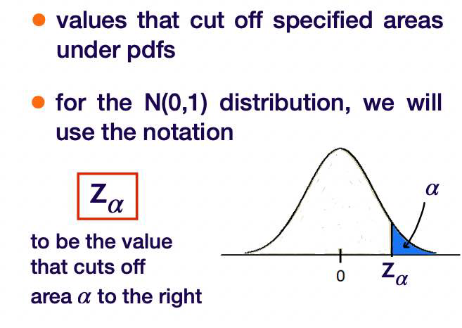
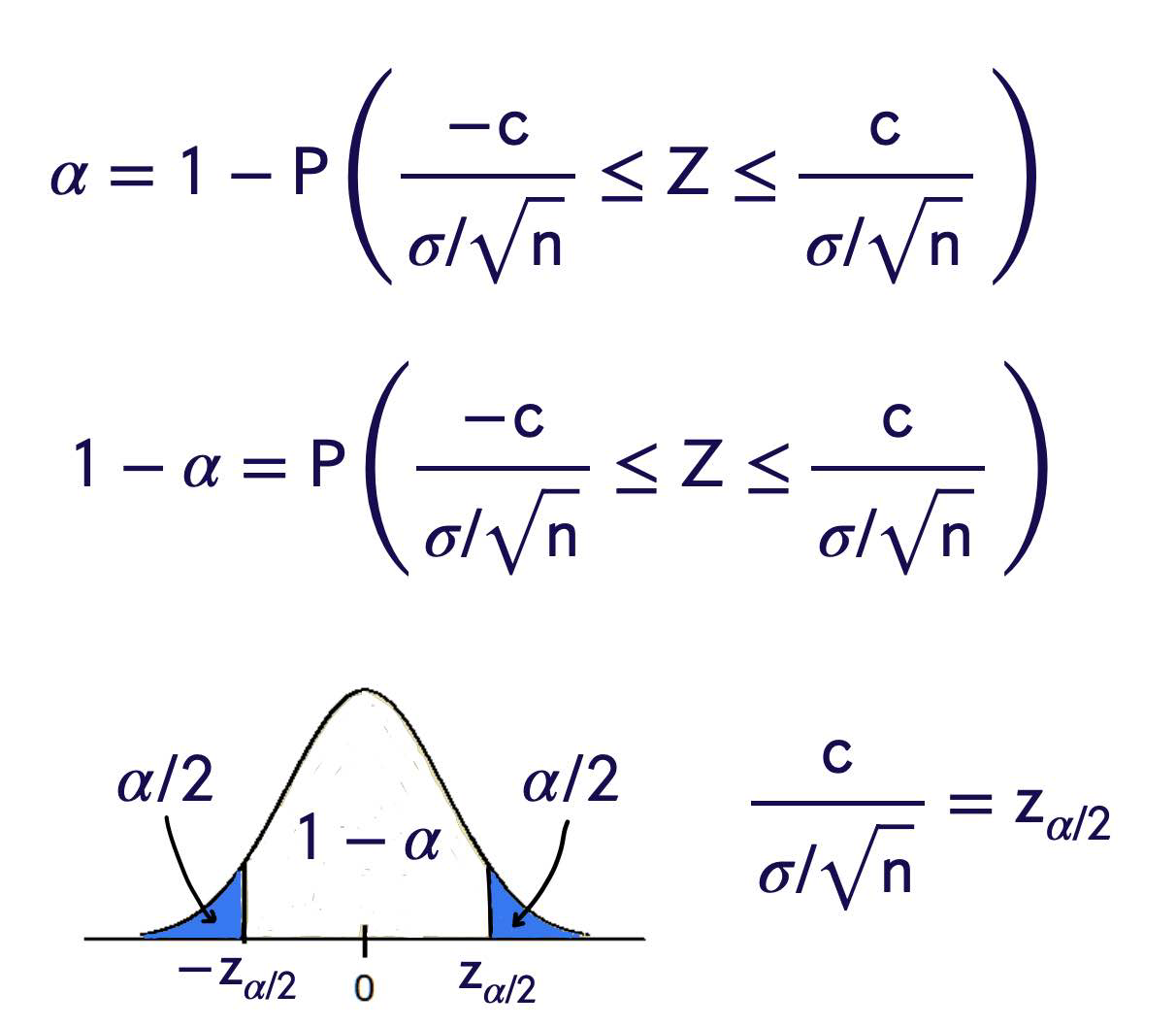
Critical values

Critical values for distributions are numbers that cut off specified areas under pdfs. For the N(0, 1) distribution, we will use the notation $z_\alpha$ to denote the value that cuts off area $\alpha$ to the right as depicted here.

Errors in Hypothesis Testing

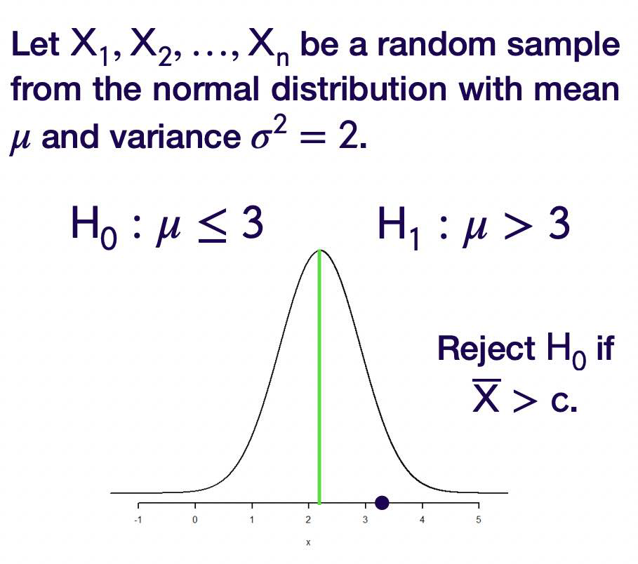
Let $X_1, X_2, \ldots, X_n$ be a random sample from the normal distribution with mean $\mu$ and variance $\sigma^2=2$

\[ H _0: \mu \leq 3 \quad H _1: \mu>3 \]

Idea: Look at $\bar{X}$ and reject $H_0$ in favor of $H _1$ if $\overline{ X }$ is “large”.
i.e. Look at $\bar{X}$ and reject $H_0$ in favor of $H _1$ if $\overline{ X }> c$ for some value $c$.

You are a potato chip manufacturer and you want to ensure that the mean amount in 15 ounce bags is at least 15 ounces. $\mathrm{H}_0: \mu \leq 15 \quad \mathrm{H}_1: \mu>15$

Type I Error

The true mean is $\leq 15$ but you concluded i was $>15$. You are going to save some money because you won’t be adding chips but you are risking a lawsuit!

Type II Error

The true mean is $> 15$ but you concluded it was $\leq 15$ . You are going to be spending money increasing the amount of chips when you didn’t have to.

Developing a Test

Let $X_1, X_2, \ldots, X_n$ be a random sample from the normal distribution with mean $\mu$ and known variance $\sigma^2$.

Consider testing the simple versus simple hypotheses

\[\begin{split} \begin{aligned} & H _0: \mu=5 \\ & H _1: \mu=3 \end{aligned} \end{split}\]

level of significance

Let $\alpha= P$ (Type I Error)
$= P \left(\right.$ Reject $H _0$ when it’s true $)$
$= P \left(\right.$ Reject $H _0$ when $\left.\mu=5\right)$

$\alpha$ is called the level of significance of the test. It is also sometimes referred to as the size of the test.

\[\begin{split} \begin{aligned} \alpha &=\max P (\text { Type I Error }) \\ &=\max _{\mu \in H _0} P \left(\text { Reject } H _0 ; \mu\right) \\ \beta &=\max P (\text { Type II Error }) \\ &=\max _{\mu \in H _1} P \left(\text { Fail to Reject } H _0 ; \mu\right) \end{aligned} \end{split}\]

Power of the test

$1-\beta$ is known as the power of the test

\[\begin{split} \begin{gathered} 1-\beta=1-\max _{\mu \in H _1} P \left(\text { Fail to Reject } H _0 ; \mu\right) \\ =\min _{\mu \in H _1}\left(1- P \left(\text { Fail to Reject } H _0 ; \mu\right)\right) \\ =\min _{\mu \in H _1} P \left(\text { Reject } H _0 ; \mu\right) \quad \begin{array}{c} \text { High power } \\ \text { is good! } \end{array} \end{gathered} \end{split}\]

Step One

Choose an estimator for μ.

\[ \widehat{\mu}=\bar{X} \]

Step Two

Choose a test statistic or Give the “form” of the test.

We are looking for evidence that $H _1$ is true.
The $N \left(3, \sigma^2\right)$ distribution takes on values from $-\infty$ to $\infty$.
$\overline{ X } \sim N \left(\mu, \sigma^2 / n \right) \Rightarrow \overline{ X }$ also takes on values from $-\infty$ to $\infty$.
It is entirely possible that $\bar{X}$ is very large even if the mean of its distribution is 3.
However, if $\bar{X}$ is very large, it will start to seem more likely that $\mu$ is larger than 3.
Eventually, a population mean of 5 will seem more likely than a population mean of 3.

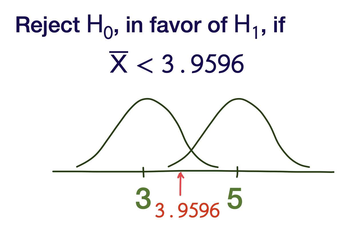
Reject $H _0$, in favor of $H _1$, if $\overline{ X }< c$ for some c to be determined.

Step Three

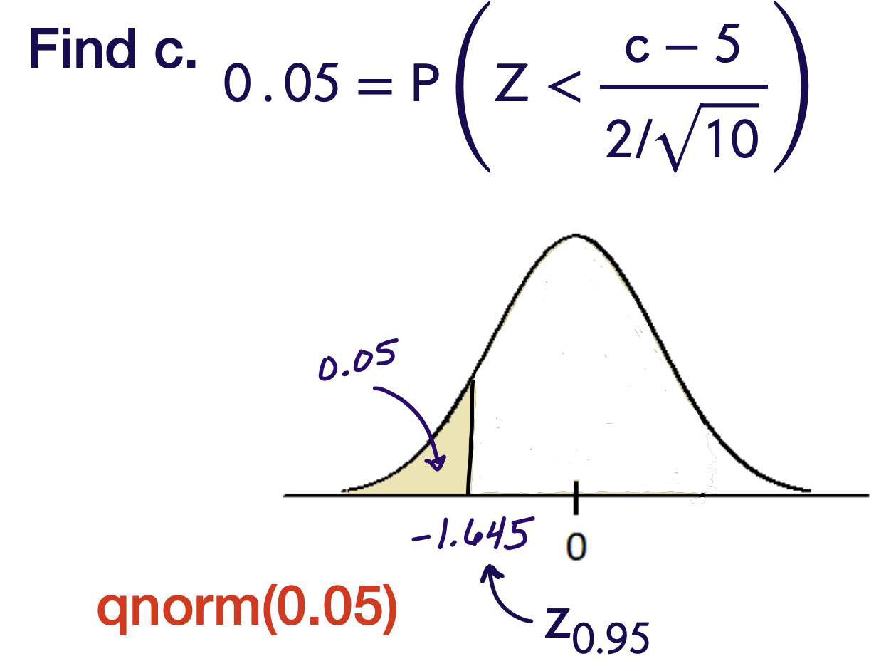
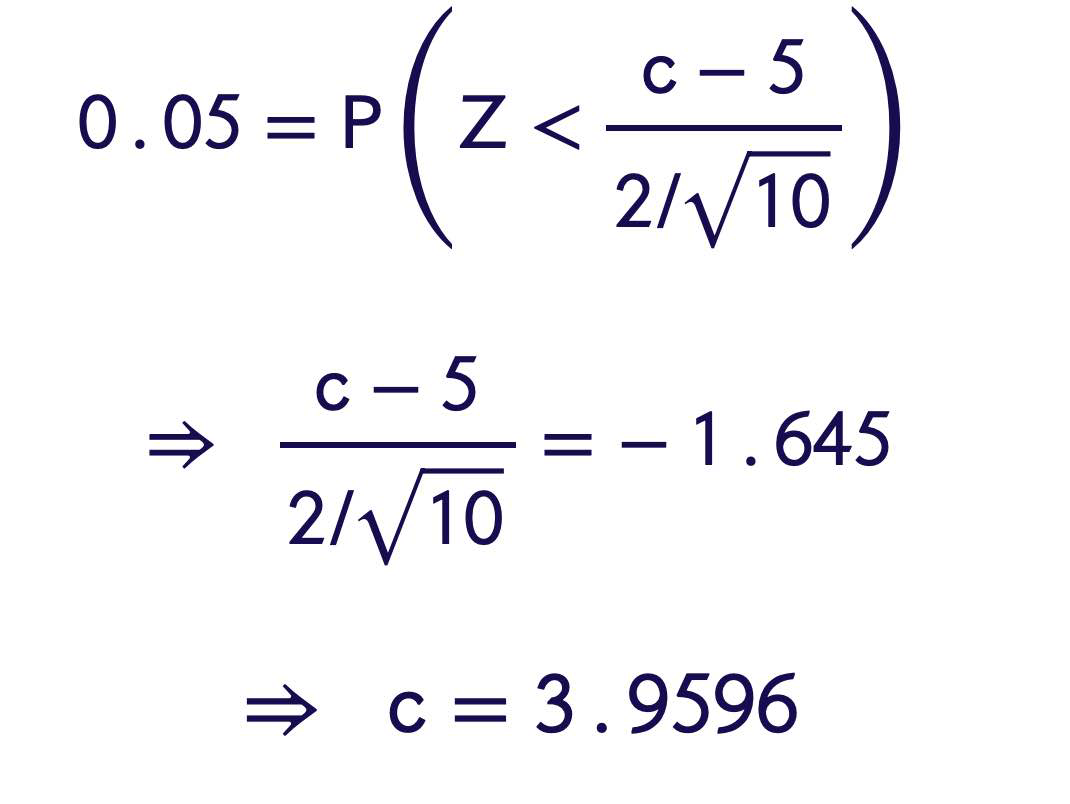
Find c.

If $c$ is too large, we are making it difficult to reject $H _0$. We are more likely to fail to reject when it should be rejected.
If $c$ is too small, we are making it to easy to reject $H _0$. We are more likely reject when it should not be rejected.

This is where $\alpha$ comes in.

\[\begin{split} \alpha&= P(Type I Error) \\ &=P( \text{Reject } H_0 \text{ when true}) \\ &=P (\overline{ X }< c \text{ when } \mu=3) \end{split}\]

Step Four

Give a conclusion!

$0.05= P ($ Type I Error)
$= P \left(\right.$ Reject $H _0$ when true $)$
$= P (\overline{ X }< \text{ c when } \mu=5)$

$ = P \left(\frac{\overline{ X }-\mu_0}{\sigma / \sqrt{ n }}<\frac{ c -5}{2 / \sqrt{10}}\right.$ when $\left.\mu=5\right)$

Formula

Let $X_1, X_2, \ldots, X_n$ be a random sample from the normal distribution with mean $\mu$ and known variance $\sigma^2$.

Consider testing the simple versus simple hypotheses

\[ H _0: \mu=\mu_0 \quad H _1: \mu=\mu_1 \]

where $\mu_0$ and $\mu_1$ are fixed and known.

\[ \begin{align}\begin{aligned}\begin{split} H_0: \mu=\mu_0 \\ H _1: \mu=\mu_1 \\ \mu_0<\mu_1 \\ \text{ Reject H0, in favor of H1 if } \\\end{split}\\\large \overline{ X }>\mu_0+ z _\alpha \frac{\sigma}{\sqrt{ n }} \end{aligned}\end{align} \]

\[ \begin{align}\begin{aligned}\begin{split} H_0: \mu=\mu_0 \\ H _1: \mu=\mu_1 \\ \mu_0>\mu_1 \\ \text{ Reject H0, in favor of H1 if } \\\end{split}\\\large \overline{ X }<\mu_0+ z_{1-\alpha} \frac{\sigma}{\sqrt{ n }} \end{aligned}\end{align} \]

Type II Error

\[\begin{split} H_0: \mu=\mu_0 \\ H _1: \mu=\mu_1 \\ \mu_0<\mu_1 \end{split}\]

\[\begin{split} \begin{aligned} & \beta= P (\text { Type II Error }) \\ =& P \left(\text { Fail to Reject } H _0 \text { when false }\right) \\ =& P \left(\overline{ X } \leq \mu_0+ z _\alpha \frac{\sigma}{\sqrt{ n }} \text { when } \mu=\mu_1\right) \\ =& P \left(\overline{ X } \leq \mu_0+ z _\alpha \frac{\sigma}{\sqrt{ n }} ; \mu_1\right) \end{aligned}\end{split}\]

\[\begin{split} \begin{aligned} \beta &= P \left(\left(\frac{\overline{X} -\mu_1}{\sigma / \sqrt{ n }}\right) \leq \frac{\mu_0+ z _\alpha \frac{\sigma}{\sqrt{ n }}-\mu_1}{\sigma / \sqrt{ n }} ; \mu_1\right) \\ &= P \left( Z \leq \frac{\mu_0+ z _\alpha \frac{\sigma}{\sqrt{ n }}-\mu_1}{\sigma / \sqrt{ n }}\right) \end{aligned} \end{split}\]

Composite vs Composite Hypothesis

\[\begin{split} \begin{aligned} & X _1, X _2, \ldots, X _{ n } \sim N \left(\mu, \sigma^2\right), \sigma^2 \text { known } \\ & H _0: \mu \leq \mu_0 \quad \text { vs } \quad H _1: \mu>\mu_0 \end{aligned} \end{split}\]

Step One Choose an estimator for μ
Step Two Choose a test statistic: Reject $H_0$ , in favor of $H_1$ if $\bar{𝖷}$ > c, where c is to be determined.
Step Three Find c.

One-Tailed Tests

Let $X_1, X_2, \ldots, X_n$ be a random sample from the normal distribution with mean $\mu$ and known variance $\sigma^2$. Consider testing the hypotheses

\[ H _0: \mu \geq \mu_0 \quad H _1: \mu<\mu_0 \]

where $\mu_0$ is fixed and known.

Step One

Choose an estimator for μ.

\[ \widehat{\mu}=\bar{X} \]

Step Two

Choose a test statistic or Give the “form” of the test.

Reject $H _0$, in favor of $H _1$, if $\overline{ X }< c$ for some c to be determined.

Step Three

Find c.

\[\begin{split} \begin{aligned} \alpha &=\max _{\mu \geq \mu_0} P (\text { Type I Error }) \\ &=\max _{\mu \geq \mu_0} P \left(\text { Reject } H _0 ; \mu\right) \\ &=\max _{\mu \geq \mu_0} P (\overline{ X }< c ; \mu) \end{aligned} \end{split}\]

\[\begin{split} \begin{aligned} \alpha &=\max _{\mu \geq \mu_0} P (\overline{ X }< c ; \mu) \\ &=\max _{\mu \geq \mu_0} P \left( Z <\frac{ c -\mu}{\sigma / \sqrt{ n }}\right) \\ &=\max _{\mu \geq \mu_0} \Phi\left(\frac{ c -\mu}{\sigma / \sqrt{ n }}\right) \end{aligned} \end{split}\]

\[\begin{split} \begin{aligned} \alpha &=\max _{\mu \geq \mu_0} P (\overline{ X }< c ; \mu) \\ &=\max _{\mu \geq \mu_0} P \left( Z <\frac{ c -\mu}{\sigma / \sqrt{ n }}\right) \\ &=\max _{\mu \geq \mu_0} \Phi\left(\frac{ c -\mu}{\sigma / \sqrt{ n }}\right) \\ \text { decreasing in } \mu \end{aligned} \end{split}\]

Step four

Reject $H _0$, in favor of $H _1$, if $$ \overline{ X }<\mu_0+ z _{1-\alpha} \frac{\sigma}{\sqrt{ n }} $$

Example

In 2019, the average health care annual premium for a family of 4 in the United States, was reported to be $\$ 6,015$.

In a more recent survey, 100 randomly sampled families of 4 reported an average annual health care premium of $\$ 6,537$. Can we say that the true average is currently greater than $\$ 6,015$ for all families of 4?

Assume that annual health care premiums are normally distributed with a standard deviation of $\$ 814$. Let $\mu$ be the true average for all families of 4.

Step Zero

Set up the hypotheses.

\[ H _0: \mu=6015 \quad H _1: \mu>6015 \]

Decide on a level of significance. $ \alpha=0.10$

Step One

Choose an estimator for $\mu$.

\[ \hat{\mu}=\bar{X} \]

Step Two

Give the form of the test. Reject $H _0$, in favor of $H _1$, if

\[ \bar{X}>c \]

for some $c$ to be determined.

Step Three

Find c.

\[\begin{split} \begin{aligned} \alpha &=\max _{\mu=\mu_0} P (\text { Type I Error; } \mu) \\ &= P \left(\text { Type I Error; } \mu_0\right) \end{aligned} \end{split}\]

\[\begin{split} \begin{aligned} &\alpha= P \left(\text { Reject } H _0 ; \mu_0\right) \text { when }\\ &= P \left(\overline{ X }> c ; \mu_0\right) \quad \text { it true!, }\\ &= P \left(\frac{\overline{ X }-\mu_0}{\sigma / \sqrt{ n }}>\frac{ c -6015}{814 / \sqrt{100}} ; \mu_0\right)\\ &=P\left(Z>\frac{c-6015}{814 / \sqrt{100}}\right) \end{aligned} \end{split}\]

\[ \frac{c-6015}{814 / \sqrt{100}}=1.28 \]

Step Four

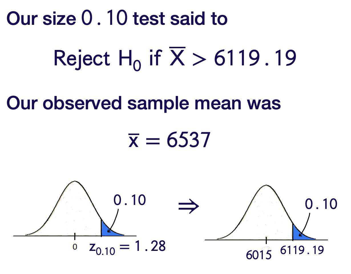
Conclusion. Reject $H _0$, in favor of $H _1$, if

\[ \bar{X}>6119.19 \]

From the data, where $\bar{x}=6537$, we reject $H _0$ in favor of $H _1$.
The data suggests that the true mean annual health care premium is greater than $\$ 6015$.

Hypothesis Testing with P-Values

Recall that p-values are defined as the following: A p-value is the probability that we observe a test statistic at least as extreme as the one we calculated, assuming the null hypothesis is true. It isn’t immediately obvious what that definition means, so let’s look at some examples to really get an idea of what p-values are, and how they work.

Let’s start very simple and say we have 5 data points: x = <1, 2, 3, 4, 5>. Let’s also assume the data were generated from some normal distribution with a known variance $\sigma$ but an unknown mean $\mu_0$. What would be a good guess for the true mean? We know that this data could come from any normal distribution, so let’s make two wild guesses:

The true mean is 100.
The true mean is 3.

Intuitively, we know that 3 is the better guess. But how do we actually determine which of these guesses is more likely? By looking at the data and asking “how likely was the data to occur, assuming the guess is true?”

What is the probability that we observed x=<1,2,3,4,5> assuming the mean is 100? Probabiliy pretty low. And because the p-value is low, we “reject the null hypothesis” that $\mu_0 = 100$.
What is the probability that we observed x=<1,2,3,4,5> assuming the mean is 3? Seems reasonable. However, something to be careful of is that p-values do not prove anything. Just because it is probable for the true mean to be 3, does not mean we know the true mean is 3. If we have a high p-value, we “fail to reject the null hypothesis” that $\mu_0 = 3$.

What do “low” and “high” mean? That is where your significance level $\alpha$ comes back into play. We consider a p-value low if the p-value is less than $\alpha$, and high if it is greater than $\alpha$.

Example

From the above example.

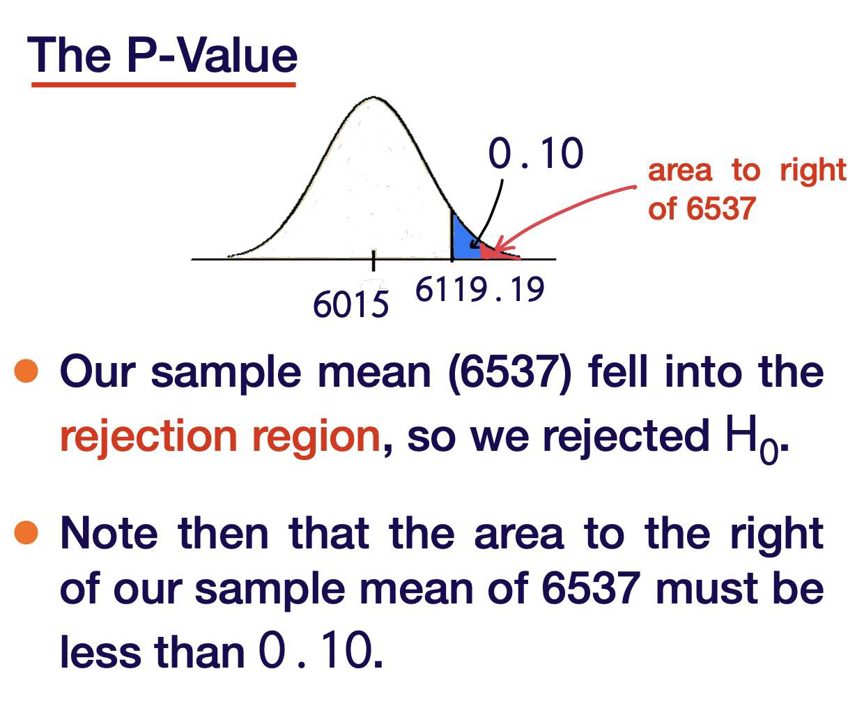
This is the $N\left(6015,814^2 / 100\right)$ pdf.
The red area is $P (\overline{ X }>6537)$.

\[\begin{split} \begin{aligned} & P (\overline{ X }>6537) \\ &\quad= P \left(\frac{\overline{ X }-\mu_0}{\sigma / \sqrt{ n }}>\frac{6537-6015}{814 / \sqrt{100}}\right) \\ &= P ( Z >6.4127) \\ &\approx 0.00000001 \quad \begin{array}{l} \text { Super small } \\ \text { and way out } \\ \text { "in the tail". } \end{array} \end{aligned} \end{split}\]

The P-Value is the area to the right (in this case) of the test statistic $\bar{X}$.
The P-value being less than $0.10$ puts $\bar{X}$ in the rejection region.
The P-value is also less than $0.05$ and $0.01$.
It looks like we will reject $H _0$ for the most typical values of $\alpha$.

Power Functions

Let $X_1, X_2, \ldots, X_n$ be a random sample from any distribution with unknown parameter $\theta$ which takes values in a parameter space $\Theta$

We ultimately want to test

\[\begin{split} \begin{aligned} & H _0: \theta \in \Theta_0 \\ & H _1: \theta \in \Theta \backslash \Theta_0 \end{aligned} \end{split}\]

where $\Theta_0$ is some subset of $\Theta$.

So in other words, if the null hypothesis was for you to test for an exponential distribution, whether lambda was between 0 and 2, the complement of that is not the rest of the real number line because the space is only non-negative values. So the complement of the interval from 0 to 2 in that space is 2 to infinity.

$\gamma(\theta)= P \left(\right.$ Reject $H _0$ when the parameter is $\left.\theta\right)$

\[ \gamma(\theta)= P \left(\text { Reject } H _0 ; \theta\right) \]

$\theta$ is an argument that can be anywhere in the parameter space $\Theta$. it could be a $\theta$ from $H _0$ it could be a $\theta$ from $H _1$

\[\begin{split} \begin{aligned} &\alpha=\max P \left(\text { Reject } H _0 \text { when true }\right) \\ &=\max _{\theta \in \Theta_0} P \left(\text { Reject } H _0 ; \theta\right) \\ &=\max _{\theta \in \Theta_0} \gamma(\theta) \longleftrightarrow \begin{array}{l} \text { Other notation } \\ \text { is } \max _{\theta \in H _0} \\ \hline \end{array} \\ & \end{aligned} \end{split}\]

Two Tailed Tests

Let $X_1, X_2, \ldots, X_n$ be a random sample from the normal distribution with mean $\mu$ and known variance $\sigma^2$.

Derive a hypothesis test of size $\alpha$ for testing

\[\begin{split} \begin{aligned} & H _0: \mu=\mu_0 \\ & H _1: \mu \neq \mu_0 \end{aligned} \end{split}\]

We will look at the sample mean $\bar{X} \ldots$ $\ldots$ and reject if it is either too high or too low.

Step One

Choose an estimator for μ.

\[ \widehat{\mu}=\bar{X} \]

Step Two

Choose a test statistic or Give the “form” of the test.

Reject $H _0$, in favor of $H _1$ if either $\overline{ X }< c$ or $\bar{X}>d$ for some $c$ and $d$ to be determined.

Easier to make it symmetric! Reject $H _0$, in favor of $H _1$ if either

\[\begin{split} \begin{aligned} &\overline{ X }>\mu_0+ c \\ &\overline{ X }<\mu_0- c \end{aligned} \end{split}\]

for some $c$ to be determined.

Step Three

Find c.

\[\begin{split} \begin{aligned} \alpha &=\max _{\mu=\mu_0} P (\text { Type I Error }) \\ &=\max _{\mu=\mu_0} P \left(\text { Reject } H _0 ; \mu\right) \\ &= P \left(\text { Reject } H _0 ; \mu_0\right) \end{aligned} \end{split}\]

\[\begin{split} \begin{aligned} &\alpha= P \left(\overline{ X }<\mu_0- c \text { or } \overline{ X }>\mu_0+ c ; \mu_0\right) \\ &=1- P \left(\mu_0- c \leq \overline{ X } \leq \mu_0+ c ; \mu_0\right) \end{aligned} \end{split}\]

\[\begin{split} \begin{gathered} \alpha=1- P \left(\frac{- c }{\sigma / \sqrt{ n }} \leq Z \leq \frac{ c }{\sigma / \sqrt{ n }}\right) \\ 1-\alpha= P \left(\frac{- c }{\sigma / \sqrt{ n }} \leq Z \leq \frac{ c }{\sigma / \sqrt{ n }}\right) \end{gathered} \end{split}\]

\[ \begin{align}\begin{aligned} \frac{c}{\sigma / \sqrt{n}}=z_{\alpha / 2}\\ c=z_{\alpha / 2} \frac{\sigma}{\sqrt{n}} \end{aligned}\end{align} \]

Step Four

Conclusion

Reject $H _0$, in favor of $H _1$, if

\[\begin{split} \begin{aligned} &\overline{ X }>\mu_0+ z _{\alpha / 2} \frac{\sigma}{\sqrt{n}} \\ &\overline{ X }<\mu_0- z _{\alpha / 2} \frac{\sigma}{\sqrt{ n }} \end{aligned} \end{split}\]

Example

In 2019, the average health care annual premium for a family of 4 in the United States, was reported to be $\$ 6,015$.

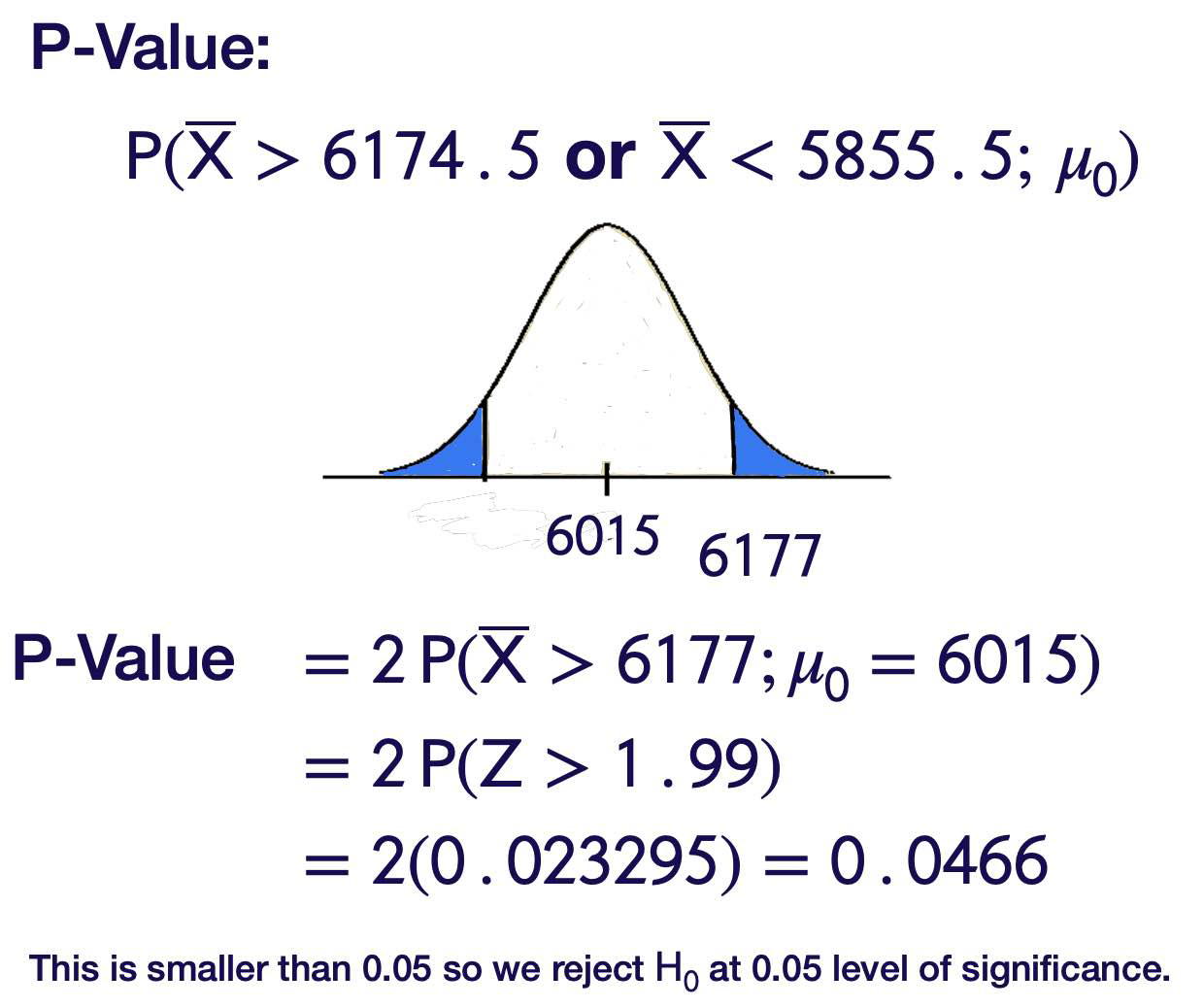
In a more recent survey, 100 randomly sampled families of 4 reported an average annual health care premium of $\$ 6,177$. Can we say that the true average, for all families of 4 , is currently different than the sample mean from 2019? $$ \sigma=814 \quad \text { Use } \alpha=0.05 $$

Assume that annual health care premiums are normally distributed with a standard deviation of $\$ 814$. Let $\mu$ be the true average for all families of 4. Hypotheses:

\[\begin{split} \begin{aligned} & H _0: \mu=6015 \\ & H _1: \mu \neq 6015 \end{aligned} \end{split}\]

\[\begin{split} \begin{aligned} &\bar{x}=6177 \quad \sigma=814 \quad n=100 \\ &z_{\alpha / 2}=z_{0.025}=1.96 \\ &\text { In R: qnorm(0.975) } \\ &6015+1.96 \frac{814}{\sqrt{100}}=6174.5 \\ &6015-1.96 \frac{814}{\sqrt{100}}=5855.5 \end{aligned} \end{split}\]

We reject $H _0$, in favor of $H _1$. The data suggests that the true current average, for all families of 4 , is different than it was in 2019.

Hypothesis Tests for Proportions

A random sample of 500 people in a certain country which is about to have a national election were asked whether they preferred “Candidate A” or “Candidate B”. From this sample, 320 people responded that they preferred Candidate A.

Let $p$ be the true proportion of the people in the country who prefer Candidate A.

Test the hypotheses $H _0: p \leq 0.65$ versus $H _1: p>0.65$ Use level of significance $0.10$. We have an estimate

\[ \hat{p}=\frac{320}{500}=\frac{16}{25} \]

The Model

Take a random sample of size $n$. Record $X_1, X_2, \ldots, X_n$ where $X_i= \begin{cases}1 & \text { person i likes Candidate A } \\ 0 & \text { person i likes Candidate B }\end{cases}$ Then $X_1, X_2, \ldots, X_n$ is a random sample from the Bernoulli distribution with parameter $p$.

Note that, with these 1’s and 0’s, $$ \begin{aligned} \hat{p} &=\frac{\# \text { in the sample who like A }}{\# \text { in the sample }} \\ &=\frac{\sum_{ i =1}^{ n } X _{ i }}{ n }=\overline{ X } \end{aligned} $$ By the Central Limit Theorem, $\hat{p}=\overline{ X }$ has, for large samples, an approximately normal distribution.

\[\begin{split} \begin{aligned} E[\hat{p}] &=E\left[X_1\right]=p \\ \operatorname{Var}[\hat{p}] &=\frac{\operatorname{Var}\left[X_1\right]}{n}=\frac{p(1-p)}{n} \end{aligned} \end{split}\]

So, $\quad \hat{p} \stackrel{\text { approx }}{\sim} N\left(p, \frac{p(1-p)}{n}\right)$

\[ \hat{p} \stackrel{\text { approx }}{\sim} N\left(p, \frac{p(1-p)}{n}\right) \]

In particular, $$ \frac{\hat{p}-p}{\sqrt{\frac{p(1-p)}{n}}} $$ behaves roughly like a $N(0,1)$ as $n$ gets large.

$n >30$ is a rule of thumb to apply to all distributions, but we can (and should!) do better with specific distributions.

$\hat{p}$ lives between 0 and 1.
The normal distribution lives between $-\infty$ and $\infty$.
However, $99.7 \%$ of the area under a $N(0,1)$ curve lies between $-3$ and 3 ,

\[\begin{split} \begin{aligned} &\hat{p} \stackrel{\text { approx }}{\sim} N\left(p, \frac{p(1-p)}{n}\right) \\ &\Rightarrow \sigma_{\hat{p}}=\sqrt{\frac{p(1-p)}{n}} \end{aligned} \end{split}\]

Go forward using normality if the interval $$ \left(\hat{p}-3 \sqrt{\frac{\hat{p}(1-\hat{p})}{n}}, \hat{p}+3 \sqrt{\frac{\hat{p}(1-\hat{p})}{n}}\right) $$ is completely contained within $[0,1]$.

Step One

Choose a statistic. $\widehat{p}=$ sample proportion for Candidate $A$

Step Two

Form of the test. Reject $H _0$, in favor of $H _1$, if $\hat{ p }> c$.

Step Three

Use $\alpha$ to find $c$ Assume normality of $\hat{p}$ ? It is a sample mean and $n>30$.

The interval $$ \left(\hat{p}-3 \sqrt{\frac{\hat{p}(1-\hat{p})}{n}}, \hat{p}+3 \sqrt{\frac{\hat{p}(1-\hat{p})}{n}}\right) $$ is $(0.5756,0.7044)$

\[\begin{split} \begin{aligned} \alpha &=\max _{p \in H_0} P (\text { Type I Error }) \\ &=\max _{p \leq 0.65} P \left(\text { Reject } H _0 ; p \right) \\ &=\max _{ p \leq 0.65} P (\hat{ p }> c ; p ) \end{aligned} \end{split}\]

\[\begin{split} \begin{aligned} \alpha &=\max _{p \leq 0.65} P\left(\frac{\hat{p}-p}{\sqrt{\frac{p(1-p)}{n}}}>\frac{c-p}{\sqrt{\frac{p(1-p)}{n}}} ; p\right) \\ & \approx \max _{p \leq 0.65} P\left(Z>\frac{c-p}{\sqrt{\frac{p(1-p)}{n}}}\right) \end{aligned} \end{split}\]

\[\begin{split} \begin{aligned} 0.10 &=\max _{p \leq 0.65} P \left(Z>\frac{c-p}{\sqrt{\frac{p(1-p)}{n}}}\right) \\ &=P\left(Z>\frac{c-0.65}{\sqrt{\frac{0.65(1-0.65)}{n}}}\right) \\ & \Rightarrow \frac{c-0.65}{\sqrt{\frac{0.65(1-0.65)}{n}}}=z_{0.10} \end{aligned} \end{split}\]

Reject $H _0$ if

\[ \hat{p}>0.65+z_{0.10} \sqrt{\frac{0.65(1-0.65)}{n}} \]

Formula

\[ \hat{p}> p +z_{0.10} \sqrt{\frac{p(1-p)}{n}} \]

T-Tests

What is a t-test, and when do we use it? A t-test is used to compare the means of one or two samples, when the underlying population parameters of those samples (mean and standard deviation) are unknown. Like a z-test, the t-test assumes that the sample follows a normal distribution. In particular, this test is useful for when we have a small sample size, as we can not use the Central Limit Theorem to use a z-test.

There are two kinds of t-tests:

One Sample t-tests
Two Sample t-tests

Let $X_1, X_2, \ldots, X_n$ be a random sample from the normal distribution with mean $\mu$ and unknown variance $\sigma^2$.

Consider testing the simple versus simple hypotheses $$ H _0: \mu=\mu_0 \quad H _1: \mu<\mu_0 $$ where $\mu_0$ is fixed and known.

Reject $H _0$, in favor of $H _1$, if

\[ \overline{ X }<\mu_0+ z _{1-\alpha} \frac{\sigma}{\sqrt{ n }} \]

unknown!This is a useless test!

It was based on the fact that

\[ \begin{align}\begin{aligned} \overline{ X } \sim N \left(\mu, \sigma^2 / n \right)\\\begin{split}\\\end{split}\\\frac{\overline{ X }-\mu}{\sigma / \sqrt{ n }} \sim N (0,1) \end{aligned}\end{align} \]

What is we use the sample standard deviation $S =\sqrt{ S ^2}$ in place of $\sigma$ ?

\[\begin{split} \begin{aligned} \frac{\overline{ X }-\mu}{ S / \sqrt{ n }} &=\frac{\overline{ X }-\mu}{\sigma / \sqrt{ n }} \cdot \frac{\sigma}{ S }=\frac{\frac{\overline{ X }-\mu}{\sigma / \sqrt{ n }}}{\frac{ S }{\sigma}} \\ &=\frac{\overline{ X }-\mu}{\sigma / \sqrt{ n }} / \sqrt{\frac{ S ^2}{\sigma^2}} \end{aligned} \end{split}\]

\[\begin{split} \begin{aligned} &\frac{\overline{ X }-\mu}{ S / \sqrt{ n }}=\frac{\overline{ X }-\mu}{\sigma / \sqrt{ n }} / \sqrt{\frac{ S ^2}{\sigma^2}} \\ &=\left(\frac{ X -\mu}{\sigma / \sqrt{ n }}\right) / \sqrt{\frac{\left(\frac{( n -1) S ^2}{\sigma^2}\right.}{ n -1}} \chi^2( n -1) \\ & N (0,1) \\ & \end{aligned} \end{split}\]

Thus,

\[ \frac{\bar{X}-\mu}{S / \sqrt{n}} \sim t(n-1) \]

Step four

Conclusion! Reject $H _0$, in favor of $H _1$, if

\[ \overline{ X }<\mu_0+ t _{1-\alpha, n -1} \frac{ S }{\sqrt{ n }} \]

Example

In 2019, the average health care annual premium for a family of 4 in the United States, was reported to be $\$ 6,015$.

In a more recent survey, 15 randomly sampled families of 4 reported an average annual health care premium of $\$ 6,033$ and a sample variance of $\$ 825$.

Can we say that the true average is currently greater than $\$ 6,015$ for all families of 4 ?

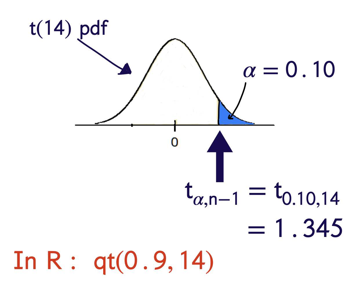
Use $\alpha=0.10$

Assume that annual health care premiums are normally distributed. Let $\mu$ be the true average for all families of 4.

Step Zero

Set up the hypotheses.

\[ H _0: \mu=6015 \quad H _1: \mu>6015 \]

Step One

Choose a test statistic

\[ \bar{X} \]

Step Two

Give the form of the test. Reject 𝖧0 , in favor of h1, if 𝟢 𝖧𝟣 𝖷 > 𝖼 where c is to be determined.

Step Three

Find c

\[\begin{split} \begin{aligned} \alpha &=\max _{\mu=\mu_0} P (\text { Type I Error }) \\ &=\max _{\mu=6015} P \left(\text { Reject } H _0 ; \mu\right) \\ &= P \left(\text { Reject } H _0 ; \mu=6015\right) \\ &= P (\overline{ X }> c ; \mu=6015) \end{aligned} \end{split}\]

\[\begin{split} \begin{gathered} \alpha= P (\overline{ X }> c ; \mu=6015) \\ = P \left(\frac{\overline{ X }-\mu_0}{ S / \sqrt{ n }}>\frac{ c -6015}{\sqrt{825} / \sqrt{15}} ; \mu=6015\right) \\ = P \left( T >\frac{ c -6015}{\sqrt{825} / \sqrt{15}}\right) \end{gathered} \end{split}\]

\[\begin{split} \begin{aligned} &\Rightarrow \frac{c-6015}{\sqrt{825} / \sqrt{15}}=1.345 \\ &\Rightarrow c=6024.98 \end{aligned} \end{split}\]

Step Four

Conclusion. Rejection Rule: Reject $H _0$, in favor of $H _1$ if

\[ \bar{X}>6024.98 \]

We had $\bar{x}=6033$ so we reject $H_0$.

There is sufficient evidence (at level $0.10$ ) in the data to suggest that the true mean annual healthcare premium cost for a family of 4 is greater than $\$ 6,015$.

P value

\[\begin{split} \begin{aligned} &\text { P-Value }= P (\overline{ X }>6033 ; \mu=6015) \\ &= P \left(\frac{\overline{ X }-\mu}{ S / \sqrt{ n }}>\frac{6033-6015}{\sqrt{825} / \sqrt{15}} ; \mu=6015\right) \\ &= P ( T >2.43) \approx 0.015 \\ &\quad \text { where } T \sim t (14) \\ &(\operatorname{In~R}: 1- pt (2.43,14) \end{aligned} \end{split}\]

Two Sample Tests for Means

Fifth grade students from two neighboring counties took a placement exam.

Group 1, from County 1, consisted of 57 students. The sample mean score for these students was $7 7 . 2$ and the true variance is known to be 15.3. Group 2, from County 2, consisted of 63 students and had a sample mean score of $75.3$ and the true variance is known to be 19.7.

From previous years of data, it is believed that the scores for both counties are normally distributed.

Derive a test to determine whether or not the two population means are the same.

\[\begin{split} \begin{aligned} & H _0: \mu_1=\mu_2 \\ & H _1: \mu_1 \neq \mu_2 \end{aligned} \end{split}\]

Suppose that $X _{1,1}, X _{1,2}, \ldots, X _{1, n _1}$ is a random sample of size $n_1$ from the normal distribution with mean $\mu_1$ and variance $\sigma_1^2$. Suppose that $X_{2,1}, X_{2,2}, \ldots, X_{2, n_2}$ is a random sample of size $n_2$ from the normal distribution with mean $\mu_2$ and variance $\sigma_2^2$.

Suppose that $\sigma_1^2$ and $\sigma_2^2$ are known and that the samples are independent.

\[\begin{split} \begin{aligned} & H _0: \mu_1=\mu_2 \quad H _1: \mu_1 \neq \mu_2 \\ & H _0: \mu_1-\mu_2=0 \\ & H _1: \mu_1-\mu_2 \neq 0 \\ & \end{aligned} \end{split}\]

Think of this as $$ \begin{gathered} \theta=0 \text { versus } \theta \neq 0 \\ \text { for } \\ \theta=\mu_1-\mu_2 \end{gathered} $$

Step one

Choose an estimator for $\theta=\mu_1-\mu_2$

\[ \hat{\theta}=\bar{X}_1-\bar{X}_2 \]

Step Two

Give the “form” of the test. Reject $H _0$, in favor of $H _1$ if either $\hat{\theta}>c$ or $\hat{\theta}<-c$ for some c to be determined.

Step Three

Find $c$ using $\alpha$ Will be working with the random variable

\[ \bar{X}_1-\bar{x}_2 \]

We need to know its distribution…

\[ \bar{X}_1-\bar{x}_2 \text{ is normally distributed.} \]

Step Three

Find c using $\alpha$.

$\bar{X}_1-\bar{X}_2$ is normally distributed

\[\begin{split} \begin{aligned} &\overline{ X }_1-\overline{ X }_2 \sim N \left(\mu_1-\mu_2, \frac{\sigma_1^2}{ n _1}+\frac{\sigma_2^2}{ n _1}\right) \\ & Z =\frac{\overline{ X }_1-\overline{ X }_2-\left(\mu_1-\mu_2\right)}{\sqrt{\frac{\sigma_1^2}{n_1}+\frac{\sigma_2^2}{n_2}}} \sim N (0,1) \end{aligned} \end{split}\]

\[\begin{split} \begin{aligned} &\alpha= P (\text { Type I Error }) \\ &\quad= P \left(\text { Reject } H _0 ; \theta=0\right) \\ &= P \left(\overline{ X }_1-\overline{ X }_2> c \text { or } \overline{ X }_1-\overline{ X }_2<- c ; \theta=0\right) \\ &=1- P \left(- c \leq \overline{ X }_1-\overline{ X }_2 \leq c ; \theta=0\right) \end{aligned} \end{split}\]

\[ =1- P \left(- c \leq \overline{ X }_1-\overline{ X }_2 \leq c ; \theta=0\right) \]

\[\begin{split} \begin{aligned} &\alpha=1- P \left(\frac{- c }{\sqrt{\frac{\sigma_1^2}{n_1}+\frac{\sigma_2^2}{n_2}}} \leq Z \leq \frac{ c }{\sqrt{\frac{\sigma_1^2}{n_1}+\frac{\sigma_2^2}{n_2}}}\right) \\ &1-\alpha= P \left(\frac{- c }{\sqrt{\frac{\sigma_1^2}{n_1}+\frac{\sigma_2^2}{n_2}}} \leq Z \leq \frac{ c }{\sqrt{\frac{\sigma_1^2}{n_1}+\frac{\sigma_2^2}{n_2}}}\right) \end{aligned} \end{split}\]

Step Four

Conclusion

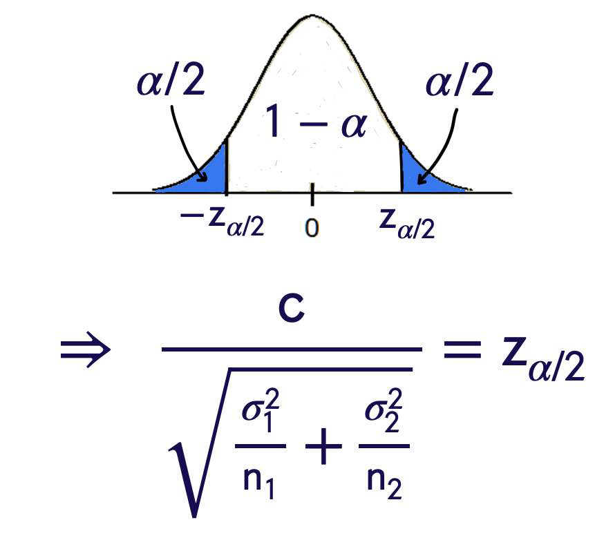
Reject $H _0$, in favor of $H _1$, if

\[ \overline{ X }_1-\overline{ X }_2> z _{\alpha / 2} \sqrt{\frac{\sigma_1^2}{ n _1}+\frac{\sigma_2^2}{ n _2}} \]

or

\[ \overline{ X }_1-\overline{ X }_2<- z _{\alpha / 2} \sqrt{\frac{\sigma_1^2}{ n _1}+\frac{\sigma_2^2}{ n _2}} \]

Example

\[\begin{split} \begin{array}{ll} n _1=57 & n _2=63 \\ \overline{ x }_1=77.2 & \overline{ x }_2=75.3 \\ \sigma_1^2=15.3 & \sigma_2^2=19.7 \end{array} \end{split}\]

Suppose that $\alpha=0.05$. $$ \begin{aligned} & z _{\alpha / 2}= z _{0.025}=1.96 \\ & z _{\alpha / 2} \sqrt{\frac{\sigma_1^2}{ n _1}+\frac{\sigma_2^2}{ n _2}}=1.49 \end{aligned} $$

\[\begin{split} \begin{aligned} & z _{\alpha / 2} \sqrt{\frac{\sigma_1^2}{ n _1}+\frac{\sigma_2^2}{ n _2}}=1.49 \\ &\overline{ x }_1-\overline{ x }_2=77.2-75.3=1.9 \end{aligned} \end{split}\]

So,

\[ \bar{x}_1-\bar{x}_2>z_{\alpha / 2} \sqrt{\frac{\sigma_1^2}{n_1}+\frac{\sigma_2^2}{n_2}} \]

and we reject $H _0$. The data suggests that the true mean scores for the counties are different!

Two Sample t-Tests for a Difference of Means

Fifth grade students from two neighboring counties took a placement exam.

Group 1, from County A, consisted of 8 students. The sample mean score for these students was $77.2$ and the sample variance is $15.3$.
Group 2, from County B, consisted of 10 students and had a sample mean score of $75.3$ and the sample variance is 19.7.

Pooled Variance

\[ S_p^2=\frac{\left(n_1-1\right) S_1^2+\left(n_2-1\right) S_2^2}{n_1+n_2-2} \]

Step Four

Reject $H _0$, in favor of $H _1$, if

\[ \bar{X}_1-\bar{X}_2>t_{\alpha / 2, n_1+n_2-2} \sqrt{\left(\frac{1}{n_1}+\frac{1}{n_2}\right) S_P^2} \]

or

\[ \bar{X}_1-\bar{X}_2<-t_{\alpha / 2, n_1+n_2-2} \sqrt{\left(\frac{1}{n_1}+\frac{1}{n_2}\right) s_P^2} \]

\[\begin{split} \begin{array}{rlr} n _1=8 & n _1=10 \\ \overline{ x }_1=77.2 & \overline{ x }_1=75.3 \\ s _1^2=15.3 & s _2^2=19.7 \\ \alpha=0.01 & t _{0.005,16}=2.92 \\ s _{ p }^2 & =\frac{\left( n _1-1\right) S _1^2+\left( n _2-1\right) S _2^2}{ n _1+ n _2-2} \\ & =17.775 \end{array} \end{split}\]

\[\begin{split} \begin{aligned} &\overline{ x }_1-\overline{ x }_2=77.2-75.3=1.9 \\ & t _{\alpha / 2, n _1+ n _2-2} \sqrt{\left(\frac{1}{ n _1}+\frac{1}{ n _2}\right) S _{ P }^2} \\ &\quad=2.92 \sqrt{\left(\frac{1}{8}+\frac{1}{10}\right)(17.775)} \\ &=5.840 \end{aligned} \end{split}\]

Since $\bar{x}_1-\bar{x}_2=1.9$ is not above $5.840$, or below $-5.840$ we fail to reject $H _0$, in favor of $H _1$ at $0.01$ level of significance.

The data do not indicate that there is a significant difference between the true mean scores for counties $A$ and $B$.

Welch’s Test and Paired Data

Two Populations: Test

\[\begin{split} \begin{aligned} & H _0: \mu_1=\mu_2 \\ & H _1: \mu_1 \neq \mu_2 \end{aligned} \end{split}\]

Suppose that $X_{1,1}, X_{1,2}, \ldots, X_{1, n_1}$ is a random sample of size $n_1$ from the normal
distribution with mean $\mu_1$ and variance $\sigma_1^2$.
Suppose that $X_{2,1}, X_{2,2}, \ldots, X_{2, n}$ is a random sample of size $n_2$ from the normal distribution with mean $\mu_2$ and variance $\sigma_2^2$.
Suppose that $\sigma_1^2$ and $\sigma_2^2$ are unknown and that the samples are independent. Don’t assume that $\sigma_1^2$ and $\sigma_2^2$ are equal!

Welch says that:

\[ \frac{\bar{X}_1-\bar{X}_2-\left(\mu_1-\mu_2\right)}{\sqrt{\frac{s_1^2}{n_1}+\frac{s_2^2}{n_2}}} \]

has an approximate t-distribution with $r$ degrees of freedom where

\[ r=\frac{S_1^2 / n_1+S_2^2 / n_2}{\frac{\left(S_1^2 / n_1\right)^2}{n_1-1}+\frac{\left(S_2^2 / n_2\right)^2}{n_2-1}} \]

rounded down.

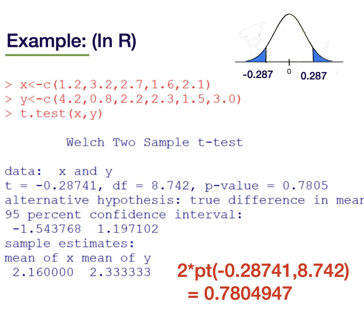
Example

A random sample of 6 students’ grades were recorded for Midterm 1 and Midterm 2. Assuming exam scores are normally distributed, test whether the true (total population of students) average grade on Midterm 2 is greater than Midterm 1. α = 0.05

Student	Midterm 1 Grade	Midterm 2 Grade
1	72	81
2	93	89
3	85	87
4	77	84
5	91	100
6	84	82

Student	Midterm 1 Grade	Midterm 2 Grade	Differences: minus 2 Midterm 1
1	72	81	9
2	93	89	-4
3	85	87	2
4	77	84	7
5	91	100.	9
6	84	82	-2

The Hypotheses: Let $\mu$ be the true average difference for all students.

\[\begin{split} \begin{aligned} & H _0: \mu=0 \\ & H _1: \mu>0 \end{aligned} \end{split}\]

This is simply a one sample t-test on the differences.

Data:

\[ 9,-4,2,7,9,-2 \]

\[ \sum x_i=23 \quad \sum x_i^2=267 \quad n=6 \]

This is simply a one sample t-test on the differences.

\[\begin{split} \begin{aligned} &\bar{x}=3.5 \\ &s^2=\frac{\sum x_i^2-\left(\sum x_i\right)^2 / n}{n-1}=32.3 \end{aligned} \end{split}\]

\[ t _{\alpha, n -1}= t _{0.05,5}=2.01 \]

Reject $H _0$, in favor of $H _1$, if

\[ \overline{ X }>\mu_0+ t _{\alpha, n -1} \frac{ S }{\sqrt{ n }} \]

3.5 > 4.6

Conclusion: We fail to reject h0 , in favor of h1 , at 0.05 level of significance.

These data do not indicate that Midterm 2 scores are higher than Midterm 1 scores

Comparing Two Population Proportions

A random sample of 500 people in a certain county which is about to have a national election were asked whether they preferred “Candidate A” or “Candidate B”. From this sample, 320 people responded that they preferred Candidate A.

A random sample of 400 people in a second county which is about to have a national election were asked whether they preferred “Candidate A” or “Candidate B”.

From this second county sample, 268 people responded that they preferred Candidate $A$.

\[\begin{split} \begin{aligned} &\hat{p}_1=\frac{320}{500}=0.64 \\ &\hat{p}_2=\frac{268}{400}=0.67 \end{aligned} \end{split}\]

Test

\[ H _0: p _1= p _2 \quad H _1: p _1 \neq p _2 \]

Change to:

\[\begin{split} \begin{aligned} & H _0: p _1- p _2=0 \\ & H _1: p _1- p _2 \neq 0 \end{aligned} \end{split}\]

Estimate $p_1-p_2$ with $\hat{p}_1-\hat{p}_2$ For large enough samples,

\[ \widehat{p}_1^{\text {approx }} N \left( p _1, \frac{ p _1\left(1- p _1\right)}{ n _1}\right) \]

and

\[ \hat{ p }_2^{\text {approx }} N \left( p _2, \frac{ p _2\left(1- p _2\right)}{ n _1}\right) \]

\[\begin{split} \begin{gathered} \hat{p}_1-\hat{p}_2 \sim N(?, ?) \\ E \left[\hat{p}_1-\hat{p}_2\right]=E\left[\hat{p}_1\right]- E \left[\hat{p}_2\right]=p_1-p_2 \\ \operatorname{Var}\left[\hat{p}_1-\hat{p}_2\right] \stackrel{\text { indep }}{=} \operatorname{Var}\left[\hat{p}_1\right]+\operatorname{Var}\left[\hat{p}_2\right] \\ =\frac{p_1\left(1-p_1\right)}{n_1}+\frac{p_2\left(1-p_2\right)}{n_2} \end{gathered} \end{split}\]

Use estimators for p1 and p2 assuming they are the same.

Call the common value p.
Estimate by putting both groups together.

\[ \hat{p}_1=\frac{320}{500}=0.64 \quad \hat{p}_2=\frac{268}{400}=0.67 \]

we have

\[\begin{split} \begin{aligned} \hat{p}=\frac{320+268}{500+400}=& \frac{588}{900}=\frac{49}{75} \\ & \approx 0.6533 \end{aligned} \end{split}\]

\[\begin{split} \begin{aligned} Z &:=\frac{\hat{p}_1-\hat{p}_2-\left(p_1-p_2\right)}{\sqrt{\frac{\hat{p}(1-\hat{p})}{n_1}+\frac{\hat{p}(1-\hat{p})}{n_2}} \sim N(0,1)} \\ =& \frac{\hat{p}_1-\hat{p}_2-\left(p_1-p_2\right)}{\sqrt{\hat{p}(1-\hat{p})\left(\frac{1}{n_1}+\frac{1}{n_2}\right)}} \end{aligned} \end{split}\]

Two-tailed test with z-critical values…

\[\begin{split} \begin{aligned} &\hat{p}=\frac{320+268}{500+400}=\frac{588}{900}=\frac{49}{75} \\ &Z=\frac{0.64-0.67-0}{\sqrt{0.6533(1-0.6533)\left(\frac{1}{500}+\frac{1}{400}\right)}} \end{aligned} \end{split}\]

= 0.9397

\[ z _{0.025}=1.96 \]

qnorm(1-0.05/2)

$Z=-0.9397$ does not fall in the rejection region!

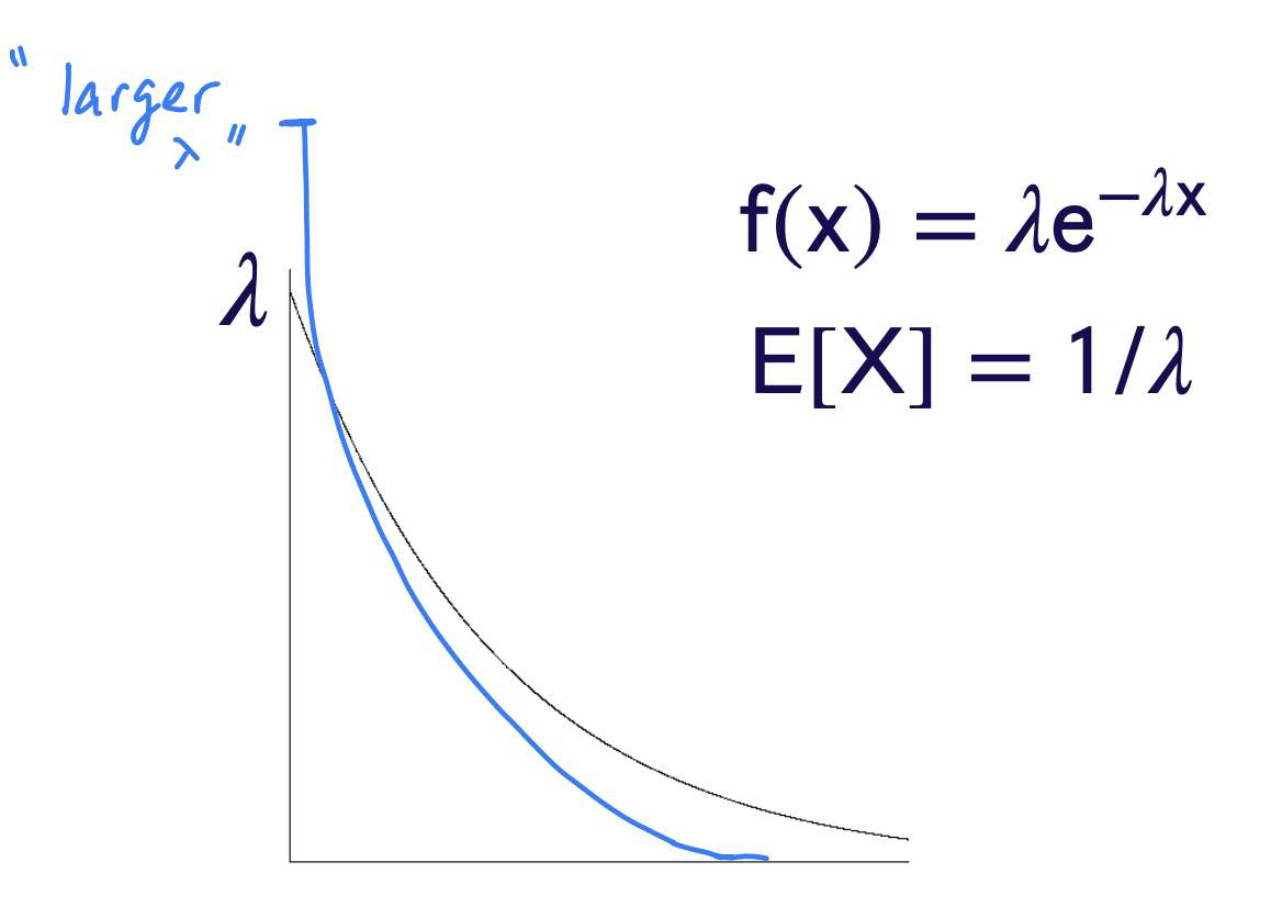
Hypothesis Tests for the Exponential

Suppose that $X_1, X_2, \ldots, X_n$ is a random sample from the exponential distribution with rate $\lambda>0$. Derive a hypothesis test of size $\alpha$ for

\[ H _0: \lambda=\lambda_0 \text { vs. } H _1: \lambda>\lambda_0 \]

What statistic should we use?

Test 1: Using the Sample Mean

Step One

Choose a statistic.

\[ \bar{x} \]

Step Two

Give the form of the test Reject 𝖧0 , in favor of h1 , if 𝖷_bar < 𝖼

for some c to be determined.

Step Three

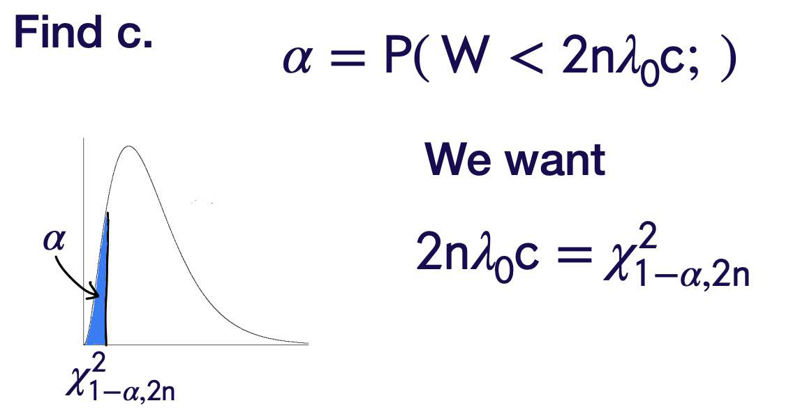
\[\begin{split} \begin{aligned} \alpha &= P (\text { Type I Error }) \\ &= P \left(\text { Reject } H _0 ; \lambda_0\right) \\ &= P \left(\overline{ X }< c ; \lambda_0\right) \end{aligned} \end{split}\]

\[\begin{split} \begin{aligned} &= P \left(2 n \lambda_0 \overline{ x }<2 n \lambda_0 c ; \lambda_0\right) \\ &= P \left( W <2 n \lambda_0 c ; \lambda_0\right) \\ \text { where } W \sim \chi^2(2 n ) \end{aligned} \end{split}\]

Step Four

Reject $H _0$, in favor of $H _1$, if

\[ \bar{x}<\frac{\chi_{1-\alpha, 2 n}^2}{2 n \lambda_0} \]

$\chi_{\alpha, n }^2$ In R, get $\chi_{0.10,6}^2$

by typing qchisq(0.90,6)

Best Test

UMP Tests

Suppose that $X_1, X_2, \ldots, X_n$ is a random sample from the exponential distribution with rate $\lambda>0$.

Derive a uniformly most powerful hypothesis test of size $\alpha$ for

\[\begin{split} \begin{array}{r} H _0: \lambda=\lambda_0 \quad \text { vs. } \quad H _1: \lambda>\lambda_0 \\ \left(\text { Was } H _1: \lambda=\lambda_1 \text { for } \lambda_1>\lambda_0\right) \end{array} \end{split}\]

Step One

Consider the simple versus simple hypotheses

\[ H _0: \lambda=\lambda_0 \quad \text { vs. } H _1: \lambda=\lambda_1 \]

for some fixed $\lambda_1>\lambda_0$.

###Steps Two, Three, and Four

Find the best test of size $\alpha$ for

\[ H _0: \lambda=\lambda_0 \text { vs. } H _1: \lambda=\lambda_1 \]

for some fixed $\lambda_1>\lambda_0$. This test is to reject $H _0$, in favor of $H _1$ if

\[ \overline{ x }<\frac{\chi_{1-\alpha, 2 n }^2}{2 n \lambda_0} \]

Note that this test does not depend on the particular value of $\lambda_1$. -It does, however, depend on the fact that $\lambda_1>\lambda_0$

The “UMP” test for

\[ H _0: \lambda=\lambda_0 \text { vs. } H _1: \lambda>\lambda_0 \]

is to reject $H_0$, in favor of $H_1$ if

\[ \overline{ x }<\frac{\chi_{1-\alpha, 2 n }^2}{2 n \lambda_0} \]

The “UMP” test for

\[ H _0: \lambda=\lambda_0 \text { vs. } H _1: \lambda<\lambda_0 \]

is to reject $H_0$, in favor of $H_1$ if

\[ \overline{ x }>\frac{\chi_{, 2 n }^2}{2 n \lambda_0} \]

Test for the Variance of the Normal Distribution

Suppose that $X_1, X_2, \ldots, X_n$ is a random sample from the normal distribution with mean $\mu$ and variance $\sigma^2$. Derive a test of size/level $\alpha$ for

\[ H _0: \sigma^2 \geq \sigma_0^2 \quad \text { vs. } H_1: \sigma^2<\sigma_0^2 \]

step 1

Choose a statistic/estimator for $\sigma^2$

\[ s^2=\frac{\sum_{i=1}^n\left(X_i-\bar{X}\right)^2}{n-1} \]

step 2

Give the form of the test. Reject $H_0$, in favor of $H_1$, if

\[ S ^2< C \]

for some $c$ to be determined.

step 3

find c using alpha

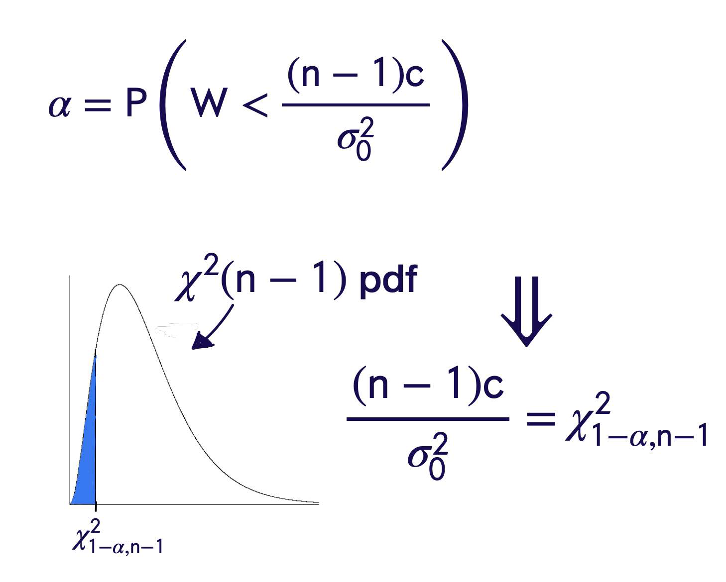
\[\begin{split} \begin{aligned} \alpha &=\max P (\text { Type I Error }) \\ &=\max _{\sigma^2 \geq \sigma_0^2} P \left(\text { Reject } H _0 ; \sigma^2\right) \\ &=\max _{\sigma^2 \geq \sigma_0^2} P \left( S ^2< c ; \sigma^2\right) \end{aligned} \end{split}\]

\[\begin{split} \begin{aligned} &= P \left(\left(\frac{( n -1) S ^2}{\sigma^2}\right) \frac{( n -1) c }{\sigma^2} ; \sigma^2\right) \\ &= P \left( W <\frac{( n -1) c }{\sigma^2}\right) \\ &\text { where } W \sim \chi^2( n -1) \end{aligned} \end{split}\]

Step 4

Reject $H _0$, in favor of $H _1$, if

\[ S^2<\frac{\sigma_0^2 \chi_{1-\alpha, n-1}^2}{n-1} \]

Example

A lawn care company has developed and wants to patent a new herbicide applicator spray nozzle. Example: For safety reasons, they need to ensure that the application is consistent and not highly variable. The company selected a random sample of 10 nozzles and measured the application rate of the herbicide in gallons per acre

The measurements were recorded as

$0.213,0.185,0.207,0.163,0.179$
$0.161,0.208,0.210,0.188,0.195$

Assuming that the application rates are normally distributed, test the following hypotheses at level $0.04$.

\[ H _0: \sigma^2=0.01 \quad H _1: \sigma^2>0.01 \]

Get sample variance in $R$.

\[\begin{split} \begin{array}{r} x<-c(0.213,0.185,0.207,0.163,0.179 \\ 0.161,0.208,0.210,0.188,0.195) \end{array} \end{split}\]

or

\[ x<-\operatorname{scan} 0 \]

Hit and then input numbers, one by one, hitting in between and <Enter $>$ at the end.

Compute variance by typing

\[ \operatorname{var}( x ) \]

or $\left(\left(\operatorname{sum}\left(x^{\wedge} 2\right)-\left(\operatorname{sum}(x)^{\wedge} 2\right) / 10\right) / 9\right.$ Result: $0.000364$

Reject $H_0$, in favor of $H_1$, if $S^2>c$.

\[\begin{split} \begin{aligned} &\alpha= P \left( S ^2> c ; \sigma^2=0.01\right) \\ &= P \left(\frac{( n -1) S ^2}{\sigma^2}>\frac{9 c }{0.01} ; \sigma^2=0.01\right) \\ &= P \left( W >\frac{9 c }{0.01}\right) \end{aligned} \end{split}\]

Reject $H _0$, in favor of $H _1$, if $S ^2> c$

\[\begin{split} \begin{gathered} 0.04= P \left( W >\frac{9 c}{0.01}\right) \\ \frac{9 c}{0.01}=\chi_{0.04,9}^2=17.61 \\ \text { qchisq(1-0.04,9) } \end{gathered} \end{split}\]

Reject $H_0$, in favor of $H_1$, if $S^2>c$

\[\begin{split} \begin{aligned} &c=(17.61)(0.01) / 9 \approx 0.0196 \\ &s^2=0.000364 \end{aligned} \end{split}\]

Fail to reject $H _0$, in favor of $H _1$, at level 0.04. There is not sufficient evidence in the data to suggest that $\sigma^2>0.01$.