Linear Algebra

Multiplying Matrices and Vectors

Multiplication of two A x B matrices a third matrix C.

\[C = AB\]

The product operation is defined by

\[C_{i,j} = \sum_{k=1} A_{i,k} B_{k,j}\]

The value at index i,j of result matrix C is given by dot product of ith row of Matrix A with jth column of Matrix

E.g

\[ \begin{align}\begin{aligned}\begin{split}A = \begin{bmatrix} 1 & 2 \\ 3 & 4 \end{bmatrix}\end{split}\\\begin{split}B = \begin{bmatrix} 2 \\ 6 \end{bmatrix}\end{split}\\C_{1,1} = \sum_{k=1} A_{1,k} B_{k,1} = 1*2 + 2*6 = 14\end{aligned}\end{align} \]

Hadamard product & element-wise product

Element wise of multiplication to generate another matrix of same dimension.

\[ \begin{align}\begin{aligned}C = A * B\\\begin{split}\begin{bmatrix} a_{11} & a_{12} & a_{13}\\ a_{21} & a_{22} & a_{23}\\ a_{31} & a_{32} & a_{33} \end{bmatrix} \circ \begin{bmatrix} b_{11} & b_{12} & b_{13}\\ b_{21} & b_{22} & b_{23}\\ b_{31} & b_{32} & b_{33} \end{bmatrix} = \begin{bmatrix} a_{11}\, b_{11} & a_{12}\, b_{12} & a_{13}\, b_{13}\\ a_{21}\, b_{21} & a_{22}\, b_{22} & a_{23}\, b_{23}\\ a_{31}\, b_{31} & a_{32}\, b_{32} & a_{33}\, b_{33} \end{bmatrix}.\end{split}\end{aligned}\end{align} \]

Dot product

The dot product for two vectors to generate scalar value.

\[a \cdot b=\sum_{i=1}^n {a}_i{b}_i={a}_1{b}_1+{a}_2{b}_2+\cdots+{a}_n{b}_n\]

Identity and Inverse Matrices

Identity Matrix

An identity matrix is a matrix that does not change any vector when we multiply that vector by that matrix.

\[\begin{split}I = \begin{bmatrix} 1 & 0 & 0 \\\\ 0 & 1 & 0 \\\\ 0 & 0 & 1 \end{bmatrix}\end{split}\]

When ‘apply’ the identity matrix to a vector the result is this same vector:

\[ \begin{align}\begin{aligned}I \cdot v = v\\\begin{split}\begin{bmatrix} 1 & 0 & 0 \\\\ 0 & 1 & 0 \\\\ 0 & 0 & 1 \end{bmatrix} \times \begin{bmatrix} x_{1} \\\\ x_{2} \\\\ x_{3} \end{bmatrix}= \begin{bmatrix} 1 \times x_1 + 0 \times x_2 + 0\times x_3 \\\\ 0 \times x_1 + 1 \times x_2 + 0\times x_3 \\\\ 0 \times x_1 + 0 \times x_2 + 1\times x_3 \end{bmatrix}= \begin{bmatrix} x_{1} \\\\ x_{2} \\\\ x_{3} \end{bmatrix}\end{split}\end{aligned}\end{align} \]

Inverse Matrix

The inverse of a matrix \(A\) is written as \(A^{-1}\).

\[{A}^{-1}{A}={I}_n\]

A matrix \(A\) is invertible if and only if there exists a matrix \(B\) such that \(AB = BA = I\).

The inverse can be found using:

• Gaussian elimination

• LU decomposition

• Gauss-Jordan elimination

Singular Matrix

A square matrix that is not invertible is called singular or degenerate. A square matrix is singular if and only if its determinant is zero

Norm

Norm is function which measure the size of vector.

• Norms are non-negative values. If you think of the norms as a length, you easily see why it can’t be negative.

• Norms are 0 if and only if the vector is a zero vector

• The triangle inequality** \(u+v \leq u+v\)

The norm is what is generally used to evaluate the error of a model.

Example

\[ \begin{align}\begin{aligned}u= \begin{bmatrix} 1 & 6 \end{bmatrix}\\v= \begin{bmatrix} 4 & 2 \end{bmatrix}\\u+v = \sqrt{(1+4)^2+(6+2)^2} = \sqrt{89} \approx 9.43\\u+v = \sqrt{1^2+6^2}+\sqrt{4^2+2^2} = \sqrt{37}+\sqrt{20} \approx 10.55\end{aligned}\end{align} \]

The p-norm (also called \(\ell_p\)) of vector x. Let p ≥ 1 be a real number.

\[ \begin{align}\begin{aligned}\left\|x\right\|_p := \left( \sum_{i=1}^n \left|x_i\right|^p\right)^{1/p}\\\left\| x \right\| _p = \left( |x_1|^p + |x_2|^p + \dotsb + |x_n|^p \right) ^{1/p}\end{aligned}\end{align} \]

• L1 norm, Where p = 1 \(\| x \|_1 = \sum_{i=1}^n |x_i|\)

• L2 norm and euclidean norm, Where p = 2 \(\left\| x \right\|_2 = \sqrt{\sum_{i=1}^n x_i^2}\)

• L-max norm, Where p = infinity

\[ \begin{align}\begin{aligned}\begin{split}u=\begin{bmatrix} 3 \\\\ 4 \end{bmatrix}\end{split}\\u =\sqrt{|3|^2+|4|^2} =\sqrt{25} =5\end{aligned}\end{align} \]

Frobenius norm

Sometimes we may also wish to measure the size of a matrix. In the context of deep learning, the most common way to do this is with the Frobenius norm.

The Frobenius norm is the square root of the sum of the squares of all the elements of a matrix.

\[ \begin{align}\begin{aligned}\|A\|_F = \sqrt{\sum_{i=1}^m \sum_{j=1}^n A_{ij}^2}\\\|A\|_\text{F} = \sqrt{\sum_{i=1}^m \sum_{j=1}^n |a_{ij}|^2}\end{aligned}\end{align} \]

The squared Euclidean norm

The squared L^2 norm is convenient because it removes the square root and we end up with the simple sum of every squared values of the vector.

The squared Euclidean norm is widely used in machine learning partly because it can be calculated with the vector operation \(x^Tx\). There can be performance gain due to the optimization

\[ \begin{align}\begin{aligned}\begin{split}x=\begin{bmatrix} 2 \\\\ 5 \\\\ 3 \\\\ 3 \end{bmatrix}\end{split}\\x^T=\begin{bmatrix} 2 & 5 & 3 & 3 \end{bmatrix}\\\begin{split}x^Tx=\begin{bmatrix} 2 & 5 & 3 & 3 \end{bmatrix} \times \begin{bmatrix} 2 \\\\ 5 \\\\ 3 \\\\ 3 \end{bmatrix}\\\\ &= 2\times 2 + 5\times 5 + 3\times 3 + 3\times 3= 47\end{split}\end{aligned}\end{align} \]

The Trace Operator

The sum of the elements along the main diagonal of a square matrix.

\[ \begin{align}\begin{aligned}\operatorname{Tr}(A) = \sum_{i=1}^n a_{ii} = a_{11} + a_{22} + \dots + a_{nn}\\\begin{split}A=\begin{bmatrix} 2 & 9 & 8 \\\\ 4 & 7 & 1 \\\\ 8 & 2 & 5 \end{bmatrix}\end{split}\\\mathrm{Tr}(A) = 2 + 7 + 5 = 14\end{aligned}\end{align} \]

Satisfies the following properties:

\[ \begin{align}\begin{aligned}\text{tr}(A) = \text{tr}(A^T)\\\text{tr}(A + B) = \text{tr}(A) + \text{tr}(B)\\\text{tr}(cA) = c\text{tr}(A)\end{aligned}\end{align} \]

Transpose

\[(A^T)_{ij} = A_{ji}\]

Satisfies the following properties:

\[(A+B)^T = A^T + B^T (AB)^T = B^TA^T (A^T)^{-1} = (A^{-1})^T\]

Diagonal matrix

A matrix where \(A_{ij} = 0\) if \(i \neq j\).

Can be written as \(\text{diag}(a)\) where \(a\) is a vector of values specifying the diagonal entries.

Diagonal matrices have the following properties:

\[ \begin{align}\begin{aligned}\text{diag}(a) + \text{diag}(b) = \text{diag}(a + b)\\\text{diag}(a) \cdot \text{diag}(b) = \text{diag}(a * b)\\\text{diag}(a)^{-1} = \text{diag}(a_1^{-1},...,a_n^{-1})\\\text{det}(\text{diag}(a)) = \prod_i{a_i}\end{aligned}\end{align} \]

Example

\[\begin{split}\begin{bmatrix} 1 & 0 & 0\\ 0 & 4 & 0\\ 0 & 0 & -3\\ 0 & 0 & 0\\ \end{bmatrix} or \begin{bmatrix} 1 & 0 & 0 & 0 & 0\\ 0 & 4 & 0& 0 & 0\\ 0 & 0 & -3& 0 & 0\end{bmatrix}\end{split}\]

The eigenvalues of a diagonal matrix are the set of its values on the diagonal.

Symmetric matrix

A square matrix \(A\) where \(A = A^T\).

\[\begin{split}\begin{bmatrix} 1 & 7 & 3 \\ 7 & 4 & 5 \\ 3 & 5 & 0 \end{bmatrix} = A^T = A\end{split}\]

Some properties of symmetric matrices are:

• All the eigenvalues of the matrix are real.

Unit Vector

A unit vector has unit Euclidean norm.

\[ \begin{align}\begin{aligned}\|x\|_2 := \sqrt{x_1^2 + \cdots + x_n^2} = 1\\\begin{split}\begin{bmatrix} 1 \\ 0 \\ 0 \end{bmatrix} = \sqrt{1^2 + 0^2 + 0^2} = 1\end{split}\end{aligned}\end{align} \]

Orthogonal Matrix or Orthonormal Vectors

Orthogonal Vectors

Two vector x and y are orthogonal if they are perpendicular to each other or dot product is equal to zero.

\[ \begin{align}\begin{aligned}\begin{split}x=\begin{bmatrix} 2\\\\ 2 \end{bmatrix}\end{split}\\\begin{split}y=\begin{bmatrix} 2\\\\ -2 \end{bmatrix}\end{split}\\\begin{split}x^Ty= \begin{bmatrix} 2 & 2 \end{bmatrix} \begin{bmatrix} 2\\\\ -2 \end{bmatrix}= \begin{bmatrix} 2\times2 + 2\times-2 \end{bmatrix}=0\end{split}\end{aligned}\end{align} \]

Orthonormal Vectors

when the norm of orthogonal vectors is the unit norm they are called orthonormal.

Orthonormal Matrix

Orthogonal matrices are important because they have interesting properties. A matrix is orthogonal if columns are mutually orthogonal and have a unit norm (orthonormal) and rows are mutually orthonormal and have unit norm.

An orthogonal matrix is a square matrix whose columns and rows are orthonormal vectors.

\[ \begin{align}\begin{aligned}A^\mathrm{T} A = A A^\mathrm{T} = I\\A^\mathrm{T}=A^{-1}\end{aligned}\end{align} \]

where AT is the transpose of A and I is the identity matrix. This leads to the equivalent characterization: matrix A is orthogonal if its transpose is equal to its inverse.

so orthogonal matrices are of interest because their inverse is very cheap to compute.

Property 1

A orthogonal matrix has this property: \(A^T A = I\).

\[ \begin{align}\begin{aligned}\begin{split}A=\begin{bmatrix} a & b\\\\ c & d \end{bmatrix} & A^T=\begin{bmatrix} a & c\\\\ b & d \end{bmatrix}\end{split}\\\begin{split}A^TA=\begin{bmatrix} a & c\\\\ b & d \end{bmatrix} \begin{bmatrix} a & b\\\\ c & d \end{bmatrix} = \begin{bmatrix} aa + cc & ab + cd\\\\ ab + cd & bb + dd \end{bmatrix}\\\\ &= \begin{bmatrix} a^2 + c^2 & ab + cd\\\\ ab + cd & b^2 + d^2 \end{bmatrix}\end{split}\\\begin{split} A^TA=\begin{bmatrix} 1 & ab + cd\\\\ ab + cd & 1 \end{bmatrix}\end{split}\\\begin{split} \begin{bmatrix} a & c \end{bmatrix} \begin{bmatrix} b\\\\ d \end{bmatrix} = ab+cd\end{split}\\\begin{split}\begin{bmatrix} a & c \end{bmatrix} \begin{bmatrix} b\\\\ d \end{bmatrix}=0\end{split}\\\begin{split}A^TA=\begin{bmatrix} 1 & 0\\\\ 0 & 1 \end{bmatrix}\end{split}\end{aligned}\end{align} \]

that the norm of the vector \(\begin{bmatrix} a & c \end{bmatrix}\) is equal to \(a^2+c^2\) (squared L^2). In addtion, we saw that the rows of A have a unit norm because A is orthogonal. This means that \(a^2+c^2=1\) and \(b^2+d^2=1\).

Property 2

We can show that if \(A^TA=I\) then \(A^T=A^{-1}\)

\[ \begin{align}\begin{aligned}(A^TA)A^{-1}={I}A^{-1}\\(A^TA)A^{-1}=A^{-1}\\A^TAA^{-1}=A^{-1}\\A^TI=A^{-1}\\A^T=A^{-1}\end{aligned}\end{align} \]

You can refer to [this question](https://math.stackexchange.com/questions/1936020/why-is-the-inverse-of-an-orthogonal-matrix-equal-to-its-transpose).

Sine and cosine are convenient to create orthogonal matrices. Let’s take the following matrix:

\[\begin{split}A=\begin{bmatrix} cos(50) & -sin(50)\\\\ sin(50) & cos(50) \end{bmatrix}\end{split}\]

Eigendecomposition

The eigendecomposition is one form of matrix decomposition (only square matrices). Decomposing a matrix means that we want to find a product of matrices that is equal to the initial matrix. In the case of the eigendecomposition, we decompose the initial matrix into the product of its eigenvectors and eigenvalues.

\[A v = \lambda v\]

Eigenvectors and eigenvalues

Now imagine that the transformation of the initial vector gives us a new vector that has the exact same direction. The scale can be different but the direction is the same. Applying the matrix didn’t change the direction of the vector. This special vector is called an eigenvector of the matrix. We will see that finding the eigenvectors of a matrix can be very useful. Imagine that the transformation of the initial vector by the matrix gives a new vector with the exact same direction. This vector is called an eigenvector of 𝐴 . This means that 𝑣 is a eigenvector of 𝐴 if 𝑣 and 𝐴𝑣 are in the same direction or to rephrase it if the vectors 𝐴𝑣 and 𝑣 are parallel. The output vector is just a scaled version of the input vector. This scalling factor is 𝜆 which is called the eigenvalue of 𝐴 .

\[ \begin{align}\begin{aligned}\begin{split}A=\begin{bmatrix} 5 & 1\\\\ 3 & 3 \end{bmatrix}\end{split}\\\begin{split}v=\begin{bmatrix} 1\\\\ 1 \end{bmatrix}\end{split}\\Av = \lambda v\\\begin{split}\begin{bmatrix} 5 & 1\\\\ 3 & 3 \end{bmatrix} \begin{bmatrix} 1\\\\ 1 \end{bmatrix}=\begin{bmatrix} 6\\\\ 6 \end{bmatrix}\end{split}\\\begin{split}6\times \begin{bmatrix} 1\\\\ 1 \end{bmatrix} = \begin{bmatrix} 6\\\\ 6 \end{bmatrix}\end{split}\end{aligned}\end{align} \]

which means that v is well an eigenvector of A. Also, the corresponding eigenvalue is lambda=6.

Another eigenvector of 𝐴 is

\[ \begin{align}\begin{aligned}\begin{split}v=\begin{bmatrix} 1\\\\ -3 \end{bmatrix}\end{split}\\\begin{split}\begin{bmatrix} 5 & 1\\\\ 3 & 3 \end{bmatrix}\begin{bmatrix} 1\\\\ -3 \end{bmatrix} = \begin{bmatrix} 2\\\\ -6 \end{bmatrix}\end{split}\\\begin{split}2 \times \begin{bmatrix} 1\\\\ -3 \end{bmatrix} = \begin{bmatrix} 2\\\\ -6 \end{bmatrix}\end{split}\end{aligned}\end{align} \]

which means that v is an eigenvector of A. Also, the corresponding eigenvalue is lambda=2.

Rescaled vectors if v is an eigenvector of A, then any rescaled vector sv is also an eigenvector of A. The eigenvalue of the rescaled vector is the same.

\[ \begin{align}\begin{aligned}\begin{split}3v=\begin{bmatrix} 3\\\\ -9 \end{bmatrix}\end{split}\\\begin{split}\begin{bmatrix} 5 & 1\\\\ 3 & 3 \end{bmatrix} \begin{bmatrix} 3\\\\ -9 \end{bmatrix} = \begin{bmatrix} 6\\\\ -18 \end{bmatrix} = 2 \times \begin{bmatrix} 3\\\\ -9 \end{bmatrix}\end{split}\end{aligned}\end{align} \]

We have well A X 3v = lambda v and the eigenvalue is still lambda = 2 .

Concatenating eigenvalues and eigenvectors

Now that we have an idea of what eigenvectors and eigenvalues are we can see how it can be used to decompose a matrix. All eigenvectors of a matrix 𝐴 can be concatenated in a matrix with each column corresponding to each eigenvector.

\[\begin{split}v=\begin{bmatrix} 1 & 1\\\\ 1 & -3 \end{bmatrix}\end{split}\]

The first column [ 1 1 ] is the eigenvector of 𝐴 with lambda=6 and the second column [ 1 -3 ] with lambda=2.

The vector \(\lambda\) can be created from all eigenvalues:

\[\begin{split}\lambda= \begin{bmatrix} 6\\\\ 2 \end{bmatrix}\end{split}\]

Then the eigendecomposition is given by

\[A=V\cdot diag(\lambda) \cdot V^{-1}\]

Converting eigenvalues and eigenvectors to a matrix A.

\[ \begin{align}\begin{aligned}\begin{split}V^{-1}=\begin{bmatrix} 0.75 & 0.25\\\\ 0.25 & -0.25 \end{bmatrix}\end{split}\\\begin{split}&V\cdot diag(\lambda) \cdot V^{-1}\\\\ &= \begin{bmatrix} 1 & 1\\\\ 1 & -3 \end{bmatrix} \begin{bmatrix} 6 & 0\\\\ 0 & 2 \end{bmatrix} \begin{bmatrix} 0.75 & 0.25\\\\ 0.25 & -0.25 \end{bmatrix}\end{split}\\\begin{split}\begin{bmatrix} 1 & 1\\\\ 1 & -3 \end{bmatrix} \begin{bmatrix} 6 & 0\\\\ 0 & 2 \end{bmatrix} = \begin{bmatrix} 6 & 2\\\\ 6 & -6 \end{bmatrix}\end{split}\\\begin{split}&\begin{bmatrix} 6 & 2\\\\ 6 & -6 \end{bmatrix} \begin{bmatrix} 0.75 & 0.25\\\\ 0.25 & -0.25 \end{bmatrix}\\\\ &= \begin{bmatrix} 6\times0.75 + (2\times0.25) & 6\times0.25 + (2\times-0.25)\\\\ 6\times0.75 + (-6\times0.25) & 6\times0.25 + (-6\times-0.25) \end{bmatrix}\\\\ &= \begin{bmatrix} 5 & 1\\\\ 3 & 3 \end{bmatrix}= A\end{split}\end{aligned}\end{align} \]

Real symmetric matrix

In the case of real symmetric matrices, the eigendecomposition can be expressed as

\[A = Q\Lambda Q^T\]

where \(Q\) is the matrix with eigenvectors as columns and \(\Lambda\) is \(diag(\lambda)\).

\[\begin{split}A=\begin{bmatrix} 6 & 2\\\\ 2 & 3 \end{bmatrix}\end{split}\]

This matrix is symmetric because \(A=A^T\). Its eigenvectors are:

\[ \begin{align}\begin{aligned}\begin{split}Q=\begin{bmatrix} 0.89442719 & -0.4472136\\\\ 0.4472136 & 0.89442719 \end{bmatrix}\end{split}\\\begin{split}\Lambda=\begin{bmatrix} 7 & 0\\\\ 0 & 2 \end{bmatrix}\end{split}\\\begin{split} Q\Lambda&=\begin{bmatrix} 0.89442719 & -0.4472136\\\\ 0.4472136 & 0.89442719 \end{bmatrix} \begin{bmatrix} 7 & 0\\\\ 0 & 2 \end{bmatrix}\\\\ &= \begin{bmatrix} 0.89442719 \times 7 & -0.4472136\times 2\\\\ 0.4472136 \times 7 & 0.89442719\times 2 \end{bmatrix}\\\\ &= \begin{bmatrix} 6.26099033 & -0.8944272\\\\ 3.1304952 & 1.78885438 \end{bmatrix}\end{split}\\\begin{split}Q^T=\begin{bmatrix} 0.89442719 & 0.4472136\\\\ -0.4472136 & 0.89442719 \end{bmatrix}\end{split}\\\begin{split} Q\Lambda Q^T&=\begin{bmatrix} 6.26099033 & -0.8944272\\\\ 3.1304952 & 1.78885438 \end{bmatrix} \begin{bmatrix} 0.89442719 & 0.4472136\\\\ -0.4472136 & 0.89442719 \end{bmatrix}\\\\ &= \begin{bmatrix} 6 & 2\\\\ 2 & 3 \end{bmatrix}\end{split}\end{aligned}\end{align} \]

Singular Value Decomposition

The eigendecomposition can be done only for square matrices. The way to go to decompose other types of matrices that can’t be decomposed with eigendecomposition is to use Singular Value Decomposition (SVD).

SVD decompose 𝐴 into 3 matrices.

\(A = U D V^T\)

U,D,V where U is a matrix with eigenvectors as columns and D is a diagonal matrix with eigenvalues on the diagonal and V is the transpose of U.

The matrices U,D,V have the following properties:

• U and V are orthogonal matrices U^T=U^{-1} and V^T=V^{-1}

• D is a diagonal matrix However D is not necessarily square.

• The columns of U are called the left-singular vectors of A while the columns of V are the right-singular vectors of A.The values along the diagonal of D are the singular values of A.

Intuition

I think that the intuition behind the singular value decomposition needs some explanations about the idea of matrix transformation. For that reason, here are several examples showing how the space can be transformed by 2D square matrices. Hopefully, this will lead to a better understanding of this statement: 𝐴 is a matrix that can be seen as a linear transformation. This transformation can be decomposed in three sub-transformations: 1. rotation, 2. re-scaling, 3. rotation. These three steps correspond to the three matrices 𝑈 , 𝐷 , and 𝑉.

SVD and eigendecomposition

Now that we understand the kind of decomposition done with the SVD, we want to know how the sub-transformations are found. The matrices 𝑈 , 𝐷 and 𝑉 can be found by transforming 𝐴 in a square matrix and by computing the eigenvectors of this square matrix. The square matrix can be obtain by multiplying the matrix 𝐴 by its transpose in one way or the other:

𝑈 corresponds to the eigenvectors of 𝐴𝐴^T 𝑉 corresponds to the eigenvectors of 𝐴^T𝐴 𝐷 corresponds to the eigenvalues 𝐴𝐴^T or 𝐴^T𝐴 which are the same.

The Moore-Penrose Pseudoinverse

We saw that not all matrices have an inverse because the inverse is used to solve system of equations. The Moore-Penrose pseudoinverse is a direct application of the SVD. the inverse of a matrix A can be used to solve the equation Ax=b.

\[A^{-1}Ax=A^{-1}b I_nx=A^{-1}b x=A^{-1}b\]

But in the case where the set of equations have 0 or many solutions the inverse cannot be found and the equation cannot be solved. The pseudoinverse is \(A^+\) where \(A^+\) is the pseudoinverse of \(A\).

\[ \begin{align}\begin{aligned}AA^+\approx I_n\\|| AA^+-I_n ||\end{aligned}\end{align} \]

The following formula can be used to find the pseudoinverse:

\[A^+= VD^+U^T\]

Principal Components Analysis (PCA)

The aim of principal components analysis (PCA) is generaly to reduce the number of dimensions of a dataset where dimensions are not completely decorelated.

Describing the problem

The problem can be expressed as finding a function that converts a set of data points from ℝ𝑛 to ℝ𝑙 . This means that we change the number of dimensions of our dataset. We also need a function that can decode back from the transformed dataset to the initial one.

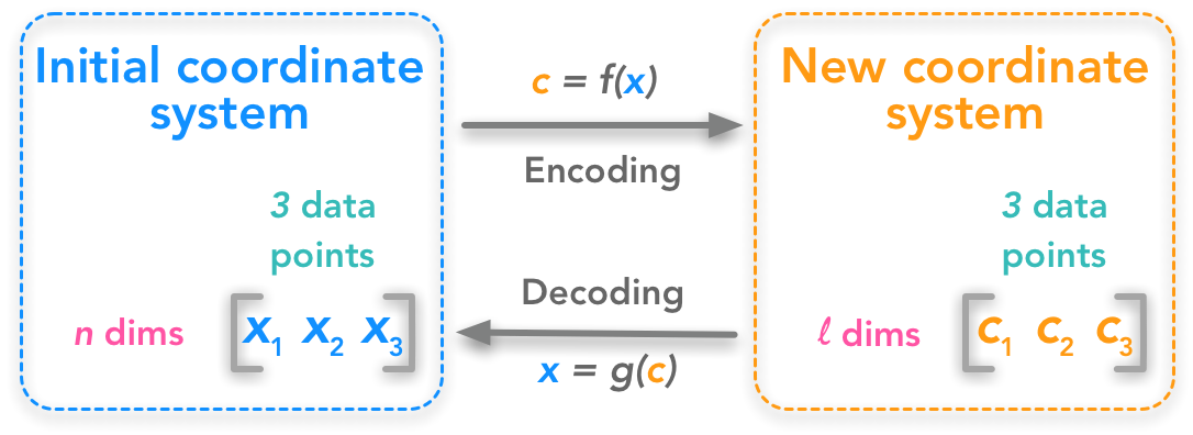
The first step is to understand the shape of the data. 𝑥(𝑖) is one data point containing 𝑛 dimensions. Let’s have 𝑚 data points organized as column vectors (one column per point):

\(x=\begin{bmatrix} x^{(1)} x^{(2)} \cdots x^{(m)} \end{bmatrix}\)

If we deploy the n dimensions of our data points we will have:

\[\begin{split}x=\begin{bmatrix} x_1^{(1)} & x_1^{(2)} & \cdots & x_1^{(m)}\\\\ x_2^{(1)} & x_2^{(2)} & \cdots & x_2^{(m)}\\\\ \cdots & \cdots & \cdots & \cdots\\\\ x_n^{(1)} & x_n^{(2)} & \cdots & x_n^{(m)} \end{bmatrix}\end{split}\]

We can also write:

\[\begin{split}x=\begin{bmatrix} x_1\\\\ x_2\\\\ \cdots\\\\ x_n \end{bmatrix}\end{split}\]

c will have the shape:

\[\begin{split}c=\begin{bmatrix} c_1\\\\ c_2\\\\ \cdots\\\\ c_l \end{bmatrix}\end{split}\]

Adding some constraints: the decoding function

The encoding function f(x) transforms x into c and the decoding function transforms back c into an approximation of x. To keep things simple, PCA will respect some constraints:

Constraint 1

The decoding function has to be a simple matrix multiplication:

$$g(c)=Dc$$

By applying the matrix D to the dataset from the new coordinates system we should get back to the initial coordinate system.

Constraint 2

The columns of D must be orthogonal.

Constraint 3

The columns of D must have unit norm.

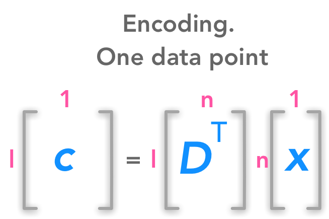
Finding the encoding function

For now we will consider only one data point. Thus we will have the following dimensions for these matrices (note that x and c are column vectors)

We want a decoding function which is a simple matrix multiplication. For that reason, we have g(c)=Dc.

We will then find the encoding function from the decoding function. We want to minimize the error between the decoded data point and the actual data point.

With our previous notation, this means reducing the distance between x and g(c). As an indicator of this distance, we will use the squared L^2 norm.

\[||x-g(c)||_2^2\]

This is what we want to minimize. Let’s call \(c^*\) the optimal c. Mathematically it can be written:

$$ c^* = argmin ||x-g(c)||_2^2 $$

This means that we want to find the values of the vector c such that \(||x-g(c)||_2^2\) is as small as possible.

the squared \(L^2\) norm can be expressed as:

$$ ||y||_2^2 = y^Ty $$

We have named the variable y to avoid confusion with our x. Here \(y=x - g(c)\) Thus the equation that we want to minimize becomes:

$$ (x - g(c))^T(x - g(c)) $$

Since the transpose respects addition we have:

$$ (x^T - g(c)^T)(x - g(c)) $$

By the distributive property we can develop:

$$ x^Tx - x^Tg(c) - g(c)^Tx + g(c)^Tg(c) $$

The commutative property tells us that \(x^Ty = y^Tx\). We can use that in the previous equation: we have \(g(c)^Tx = x^Tg(c)\). So the equation becomes:

$$ x^Tx -x^Tg(c) -x^Tg(c) + g(c)^Tg(c) = x^Tx -2x^Tg(c) + g(c)^Tg(c) $$

The first term \(x^Tx\) does not depends on c and since we want to minimize the function according to c we can just get off this term. We simplify to:

$$ c^* = arg min -2x^T g(c) + g(c)^T g(c) $$

Since \(g(c)=Dc\):

$$ c^* = arg min -2x^T Dc + (Dc)^T Dc $$

With \((Dc)^T = c^T D^T\), we have:

$$ c^* = arg min -2x^T Dc + c^T D^T Dc $$

As we knew, \(D^T D= I_l\) because D is orthogonal. and their columns have unit norm. We can replace in the equation:

$$ c^* = arg min -2x^T Dc + c^T I_l c $$

$$ c^* = arg min -2x^T Dc + c^T c $$

Minimizing the function

Now the goal is to find the minimum of the function −2𝑥T𝐷𝑐+𝑐T𝑐. One widely used way of doing that is to use the gradient descent algorithm. The main idea is that the sign of the derivative of the function at a specific value of 𝑥 tells you if you need to increase or decrease 𝑥 to reach the minimum. When the slope is near 0 , the minimum should have been reached.

Its mathematical notation is ∇𝑥𝑓(𝑥).

Here we want to minimize through each dimension of c. We are looking for a slope of 0.