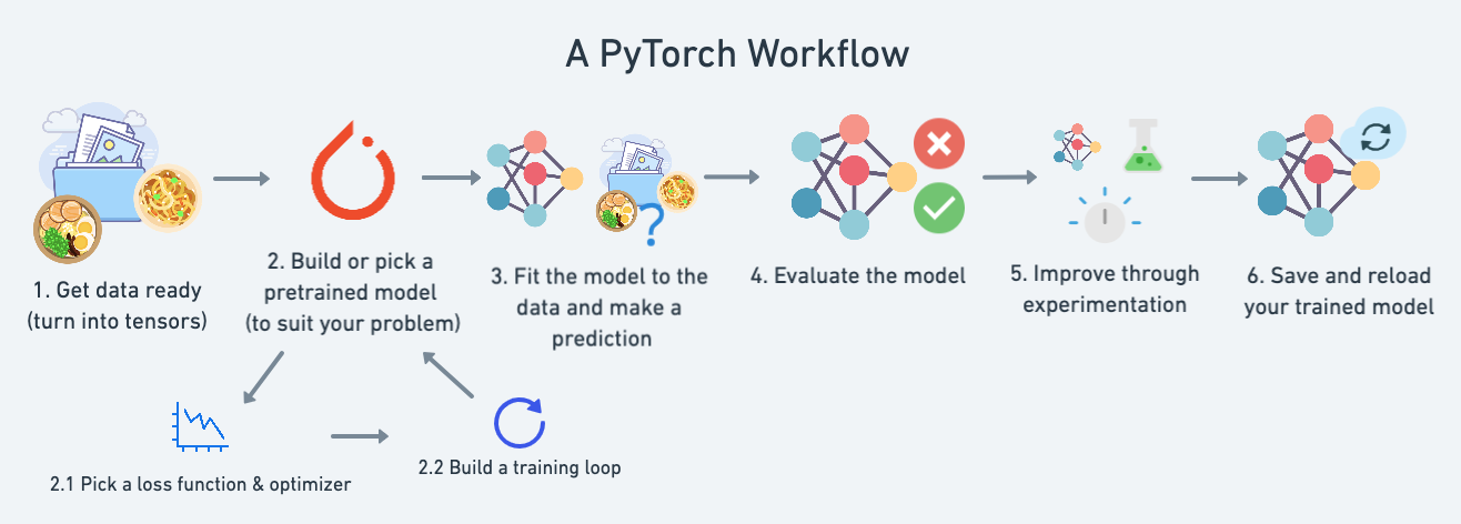
Pytorch Workflow
The essence of machine learning and deep learning is to take some data from the past, build an algorithm (like a neural network) to discover patterns in it and use the discoverd patterns to predict the future.
import torch
import torch.nn as nn
import matplotlib.pyplot as plt

torch.__version__
'2.2.2+cu121'
Data preparing and loading
I want to stress that “data” in machine learning can be almost anything you can imagine
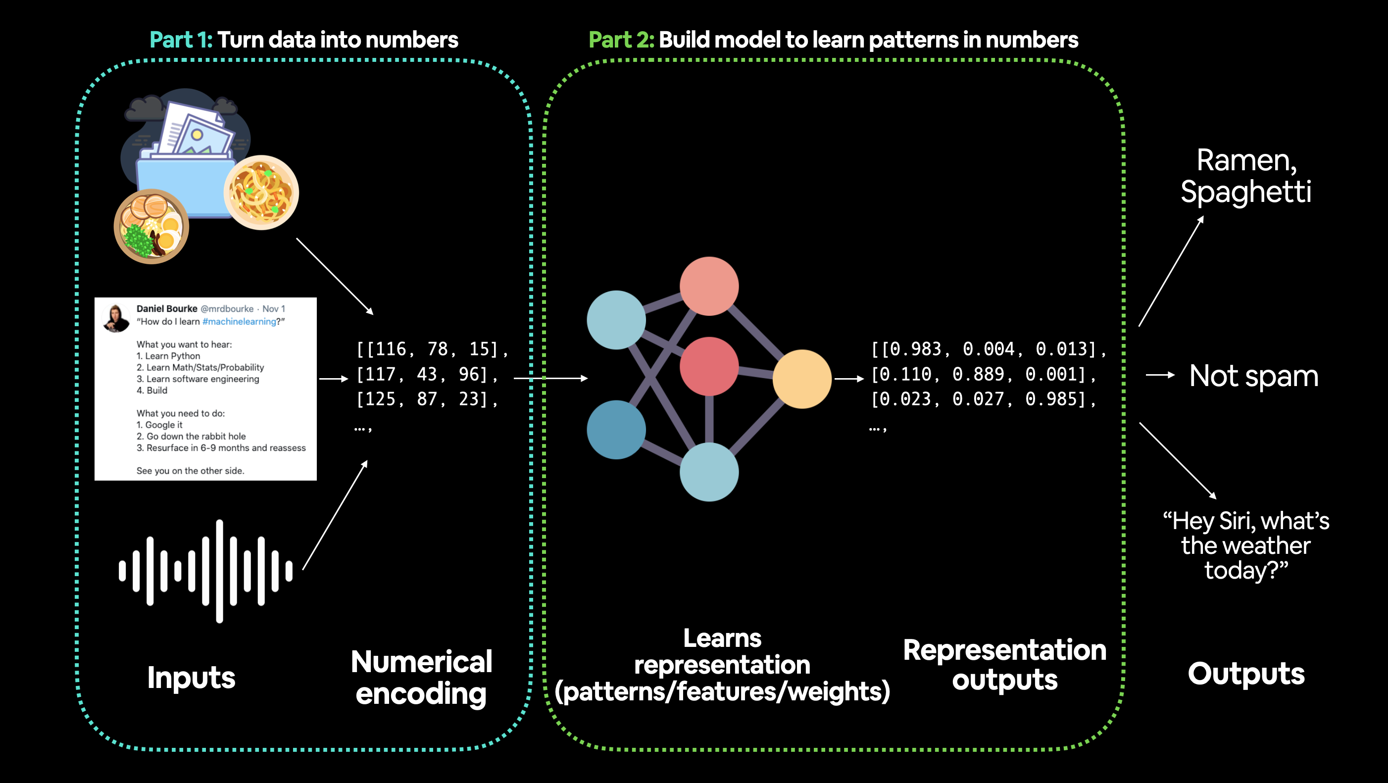
Machine learning is a game of two parts:
Turn your data, whatever it is, into numbers (a representation).
Pick or build a model to learn the representation as best as possible.
# Create *known* parameters
weight = 0.7
bias = 0.3

# Create data
start = 0
end = 1
step = 0.02
X = torch.arange(start, end, step).unsqueeze(dim=1)
y = weight * X + bias

X[:10], y[:10]
(tensor([[0.0000],
         [0.0200],
         [0.0400],
         [0.0600],
         [0.0800],
         [0.1000],
         [0.1200],
         [0.1400],
         [0.1600],
         [0.1800]]),
 tensor([[0.3000],
         [0.3140],
         [0.3280],
         [0.3420],
         [0.3560],
         [0.3700],
         [0.3840],
         [0.3980],
         [0.4120],
         [0.4260]]))
# Create train/test split
train_split = int(0.8 * len(X)) # 80% of data used for training set, 20% for testing
print(train_split)
X_train, y_train = X[:train_split], y[:train_split]
X_test, y_test = X[train_split:], y[train_split:]

len(X_train), len(y_train), len(X_test), len(y_test)
40
(40, 40, 10, 10)
def plot_predictions(train_data=X_train,
                     train_labels=y_train,
                     test_data=X_test,
                     test_labels=y_test,
                     predictions=None):
  """
  Plots training data, test data and compares predictions.
  """
  plt.figure(figsize=(10, 7))

  # Plot training data in blue
  plt.scatter(train_data, train_labels, c="b", s=4, label="Training data")

  # Plot test data in green
  plt.scatter(test_data, test_labels, c="g", s=4, label="Testing data")

  if predictions is not None:
    # Plot the predictions in red (predictions were made on the test data)
    plt.scatter(test_data, predictions, c="r", s=4, label="Predictions")

  # Show the legend
  plt.legend(prop={"size": 14});
plot_predictions()

Build model
Now we’ve got some data, let’s build a model to use the blue dots to predict the green dots.
Let’s replicate a standard linear regression model using pure PyTorch.
# Create a Linear Regression model class
class LinearRegressionModel(nn.Module): # <- almost everything in PyTorch is a nn.Module (think of this as neural network lego blocks)
    def __init__(self):
        super().__init__()
        self.weights = nn.Parameter(torch.randn(1, # <- start with random weights (this will get adjusted as the model learns)
                                                dtype=torch.float), # <- PyTorch loves float32 by default
                                   requires_grad=True) # <- can we update this value with gradient descent?)

        self.bias = nn.Parameter(torch.randn(1, # <- start with random bias (this will get adjusted as the model learns)
                                            dtype=torch.float), # <- PyTorch loves float32 by default
                                requires_grad=True) # <- can we update this value with gradient descent?))

    # Forward defines the computation in the model
    def forward(self, x: torch.Tensor) -> torch.Tensor: # <- "x" is the input data (e.g. training/testing features)
        return self.weights * x + self.bias # <- this is the linear regression formula (y = m*x + b)
# Set manual seed since nn.Parameter are randomly initialzied
torch.manual_seed(42)

# Create an instance of the model (this is a subclass of nn.Module that contains nn.Parameter(s))
model_0 = LinearRegressionModel()

# Check the nn.Parameter(s) within the nn.Module subclass we created
list(model_0.parameters())
[Parameter containing:
 tensor([0.3367], requires_grad=True),
 Parameter containing:
 tensor([0.1288], requires_grad=True)]
We can also get the state (what the model contains) of the model using .state_dict().
# List named parameters
model_0.state_dict()
OrderedDict([('weights', tensor([0.3367])), ('bias', tensor([0.1288]))])
Notice how the values for weights and bias from model_0.state_dict() come out as random float tensors?
This is becuase we initialized them above using torch.randn().
Essentially we want to start from random parameters and get the model to update them towards parameters that fit our data best (the hardcoded weight and bias values we set when creating our straight line data).
torch.inference_mode()
To check this we can pass it the test data X_test to see how closely it predicts y_test.
When we pass data to our model, it’ll go through the model’s forward() method and produce a result using the computation
# Make predictions with model
with torch.inference_mode():
    y_preds = model_0(X_test)

# Note: in older PyTorch code you might also see torch.no_grad()
# with torch.no_grad():
#   y_preds = model_0(X_test)
You probably noticed we used torch.inference_mode() as a context manager (that’s what the with torch.inference_mode(): is) to make the predictions.
As the name suggests, torch.inference_mode() is used when using a model for inference (making predictions).
torch.inference_mode() turns off a bunch of things (like gradient tracking, which is necessary for training but not for inference) to make forward-passes (data going through the forward() method) faster.
# Check the predictions
print(f"Number of testing samples: {len(X_test)}")
print(f"Number of predictions made: {len(y_preds)}")
print(f"Predicted values:\n{y_preds}")
Number of testing samples: 10
Number of predictions made: 10
Predicted values:
tensor([[0.3982],
        [0.4049],
        [0.4116],
        [0.4184],
        [0.4251],
        [0.4318],
        [0.4386],
        [0.4453],
        [0.4520],
        [0.4588]])
plot_predictions(predictions=y_preds)

y_test - y_preds

# This make sense though when you remember our model is just using random parameter values to make predictions.
tensor([[0.4618],
        [0.4691],
        [0.4764],
        [0.4836],
        [0.4909],
        [0.4982],
        [0.5054],
        [0.5127],
        [0.5200],
        [0.5272]])
loss function and optimizer in PyTorch
For our model to update its parameters on its own, we’ll need to add a few more things to our recipe.
And that’s a loss function as well as an optimizer.
Let’s create a loss function and an optimizer we can use to help improve our model.
Depending on what kind of problem you’re working on will depend on what loss function and what optimizer you use.
However, there are some common values, that are known to work well such as the SGD (stochastic gradient descent) or Adam optimizer. And the MAE (mean absolute error) loss function for regression problems (predicting a number) or binary cross entropy loss function for classification problems (predicting one thing or another).
For our problem, since we’re predicting a number, let’s use MAE (which is under torch.nn.L1Loss()) in PyTorch as our loss function.
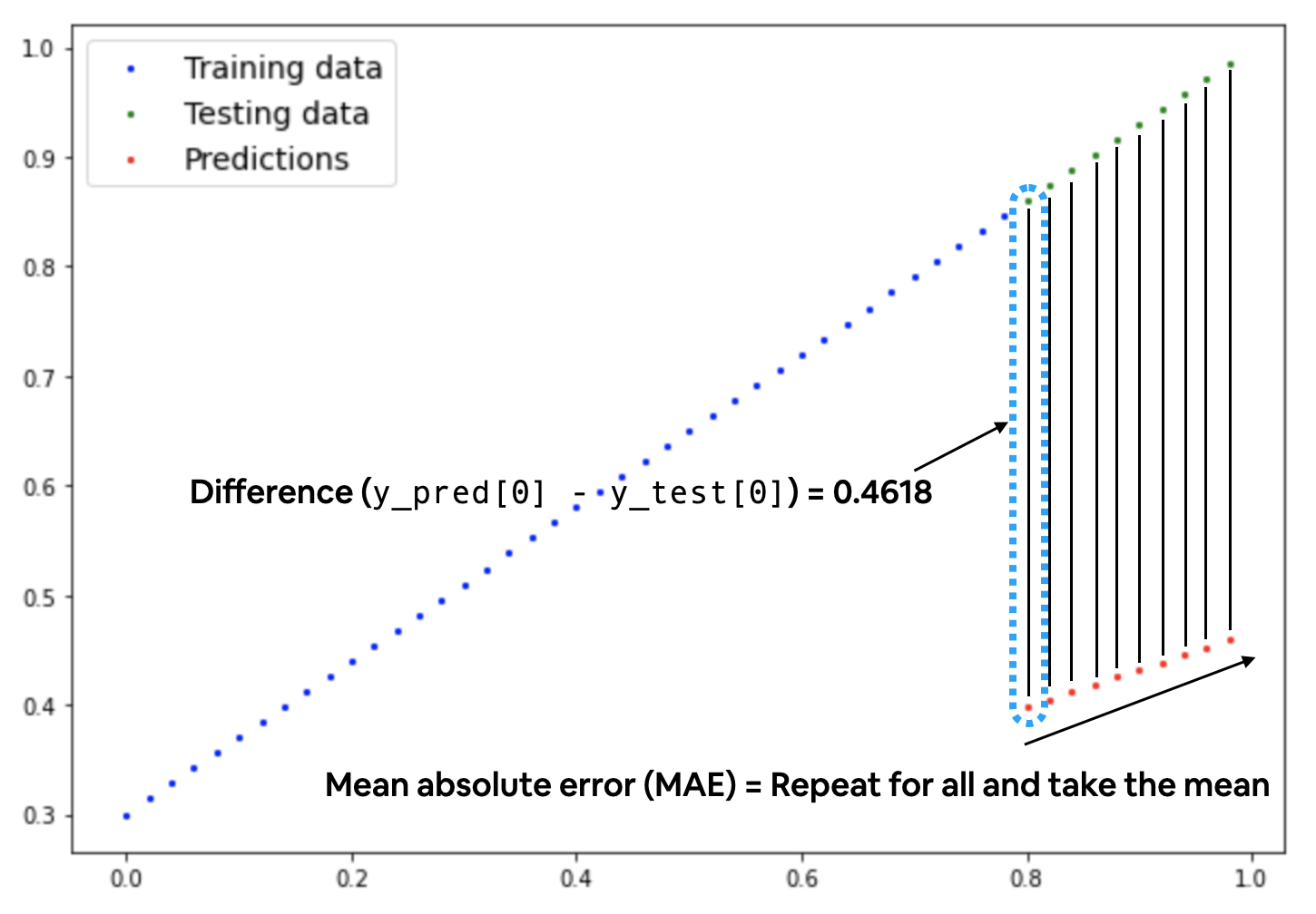
Mean absolute error (MAE, in PyTorch: torch.nn.L1Loss) measures the absolute difference between two points (predictions and labels) and then takes the mean across all examples.
And we’ll use SGD, torch.optim.SGD(params, lr) where:
params is the target model parameters you’d like to optimize (e.g. the weights and bias values we randomly set before).
lr is the learning rate you’d like the optimizer to update the parameters at, higher means the optimizer will try larger updates (these can sometimes be too large and the optimizer will fail to work), lower means the optimizer will try smaller updates (these can sometimes be too small and the optimizer will take too long to find the ideal values).
The learning rate is considered a hyperparameter (because it’s set by a machine learning engineer). Common starting values for the learning rate are 0.01, 0.001, 0.0001, however, these can also be adjusted over time (this is called learning rate scheduling). Woah, that’s a lot, let’s see it in code.
# Create the loss function
loss_fn = nn.L1Loss() # MAE loss is same as L1Loss

# Create the optimizer
optimizer = torch.optim.SGD(params=model_0.parameters(), # parameters of target model to optimize
                            lr=0.01) # learning rate (how much the optimizer should change parameters at each step, higher=more (less stable), lower=less (might take a long time))
Creating an optimization loop in PyTorch
The training loop involves the model going through the training data and learning the relationships between the features and labels.
The testing loop involves going through the testing data and evaluating how good the patterns are that the model learned on the training data (the model never see’s the testing data during training).
Number |
Step name |
What does it do? |
Code example |
|---|---|---|---|
1 |
Forward pass |
The model goes through all of the training data once, performing its |
|
2 |
Calculate the loss |
The model’s outputs (predictions) are compared to the ground truth and evaluated to see how wrong they are. |
|
3 |
Zero gradients |
The optimizers gradients are set to zero (they are accumulated by default) so they can be recalculated for the specific training step. |
|
4 |
Perform backpropagation on the loss |
Computes the gradient of the loss with respect for every model parameter to be updated (each parameter with |
|
5 |
Update the optimizer (gradient descent) |
Update the parameters with |
|
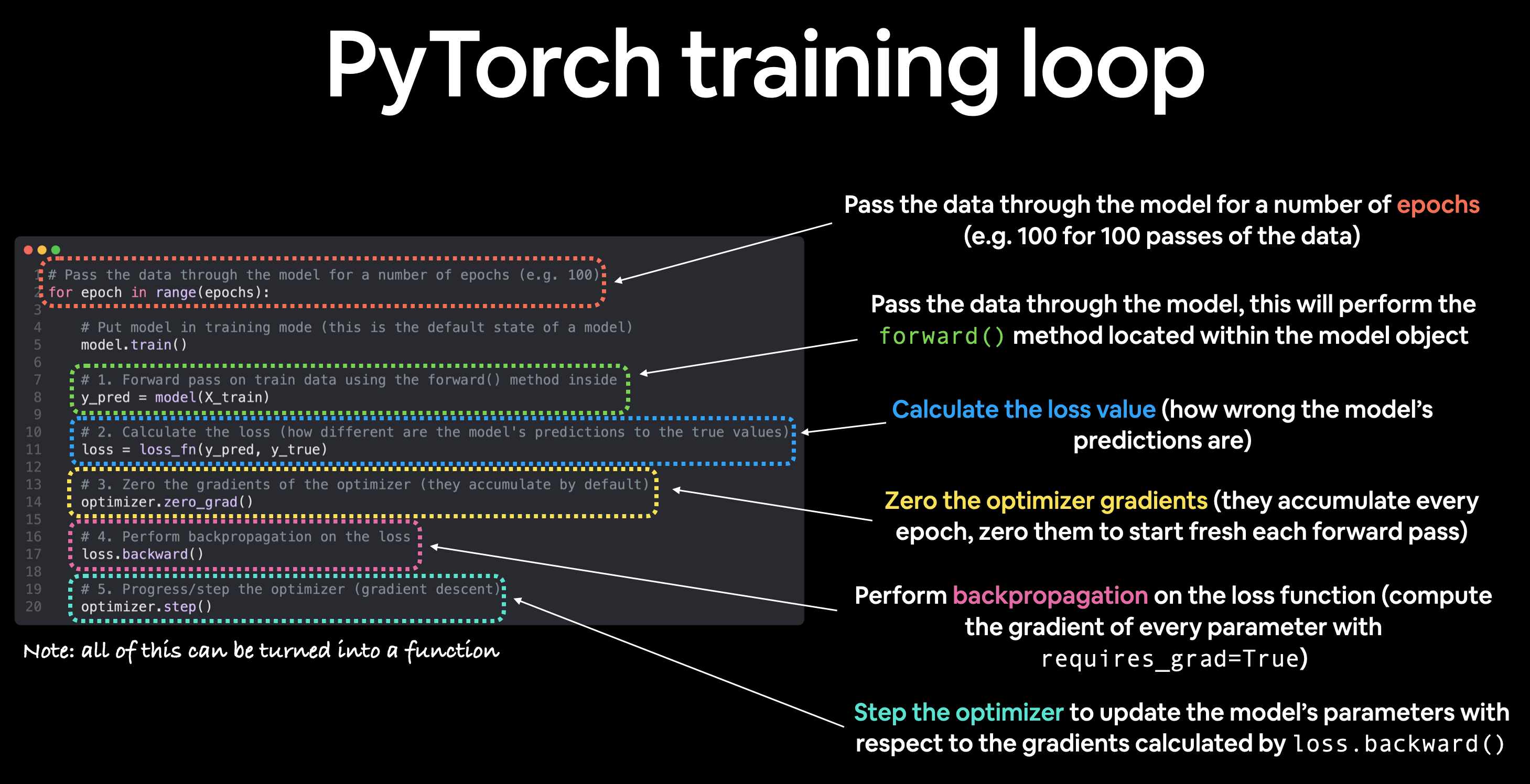
Note: The above is just one example of how the steps could be ordered or described. With experience you’ll find making PyTorch training loops can be quite flexible.
And on the ordering of things, the above is a good default order but you may see slightly different orders. Some rules of thumb:
Calculate the loss (
loss = ...) before performing backpropagation on it (loss.backward()).Zero gradients (
optimizer.zero_grad()) before stepping them (optimizer.step()).Step the optimizer (
optimizer.step()) after performing backpropagation on the loss (loss.backward()).
For resources to help understand what’s happening behind the scenes with backpropagation and gradient descent, see the extra-curriculum section.
PyTorch testing loop
As for the testing loop (evaluating our model), the typical steps include:
Number |
Step name |
What does it do? |
Code example |
|---|---|---|---|
1 |
Forward pass |
The model goes through all of the training data once, performing its |
|
2 |
Calculate the loss |
The model’s outputs (predictions) are compared to the ground truth and evaluated to see how wrong they are. |
|
3 |
Calulate evaluation metrics (optional) |
Alongisde the loss value you may want to calculate other evaluation metrics such as accuracy on the test set. |
Custom functions |
Notice the testing loop doesn’t contain performing backpropagation (loss.backward()) or stepping the optimizer (optimizer.step()), this is because no parameters in the model are being changed during testing, they’ve already been calculated. For testing, we’re only interested in the output of the forward pass through the model.
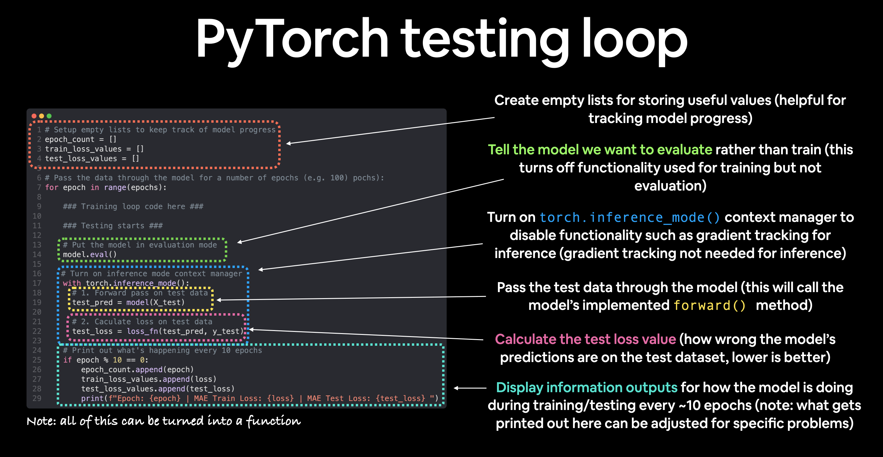
Let’s put all of the above together and train our model for 100 epochs (forward passes through the data) and we’ll evaluate it every 10 epochs.
torch.manual_seed(42)

# Set the number of epochs (how many times the model will pass over the training data)
epochs = 100

# Create empty loss lists to track values
train_loss_values = []
test_loss_values = []
epoch_count = []

for epoch in range(epochs):
    ### Training

    # Put model in training mode (this is the default state of a model)
    model_0.train()

    # 1. Forward pass on train data using the forward() method inside
    y_pred = model_0(X_train)
    # print(y_pred)

    # 2. Calculate the loss (how different are our models predictions to the ground truth)
    loss = loss_fn(y_pred, y_train)

    # 3. Zero grad of the optimizer
    optimizer.zero_grad()

    # 4. Loss backwards
    loss.backward()

    # 5. Progress the optimizer
    optimizer.step()

    ### Testing

    # Put the model in evaluation mode
    model_0.eval()

    with torch.inference_mode():
      # 1. Forward pass on test data
      test_pred = model_0(X_test)

      # 2. Caculate loss on test data
      test_loss = loss_fn(test_pred, y_test.type(torch.float)) # predictions come in torch.float datatype, so comparisons need to be done with tensors of the same type

      # Print out what's happening
      if epoch % 10 == 0:
            epoch_count.append(epoch)
            train_loss_values.append(loss.detach().numpy())
            test_loss_values.append(test_loss.detach().numpy())
            print(f"Epoch: {epoch} | MAE Train Loss: {loss} | MAE Test Loss: {test_loss} ")
Epoch: 0 | MAE Train Loss: 0.31288138031959534 | MAE Test Loss: 0.48106518387794495
Epoch: 10 | MAE Train Loss: 0.1976713240146637 | MAE Test Loss: 0.3463551998138428
Epoch: 20 | MAE Train Loss: 0.08908725529909134 | MAE Test Loss: 0.21729660034179688
Epoch: 30 | MAE Train Loss: 0.053148526698350906 | MAE Test Loss: 0.14464017748832703
Epoch: 40 | MAE Train Loss: 0.04543796554207802 | MAE Test Loss: 0.11360953003168106
Epoch: 50 | MAE Train Loss: 0.04167863354086876 | MAE Test Loss: 0.09919948130846024
Epoch: 60 | MAE Train Loss: 0.03818932920694351 | MAE Test Loss: 0.08886633068323135
Epoch: 70 | MAE Train Loss: 0.03476089984178543 | MAE Test Loss: 0.0805937647819519
Epoch: 80 | MAE Train Loss: 0.03132382780313492 | MAE Test Loss: 0.07232122868299484
Epoch: 90 | MAE Train Loss: 0.02788739837706089 | MAE Test Loss: 0.06473556160926819
# Plot the loss curves
plt.plot(epoch_count, train_loss_values, label="Train loss")
plt.plot(epoch_count, test_loss_values, label="Test loss")
plt.title("Training and test loss curves")
plt.ylabel("Loss")
plt.xlabel("Epochs")
plt.legend()
<matplotlib.legend.Legend at 0x7f76249e61d0>

# Find our model's learned parameters
print("The model learned the following values for weights and bias:")
print(model_0.state_dict())
print("\nAnd the original values for weights and bias are:")
print(f"weights: {weight}, bias: {bias}")
The model learned the following values for weights and bias:
OrderedDict([('weights', tensor([0.5784])), ('bias', tensor([0.3513]))])

And the original values for weights and bias are:
weights: 0.7, bias: 0.3
Wow! How cool is that?
Our model got very close to calculate the exact original values for weight and bias (and it would probably get even closer if we trained it for longer).
Exercise: Try changing the epochs value above to 200, what happens to the loss curves and the weights and bias parameter values of the model?
It’d likely never guess them perfectly (especially when using more complicated datasets) but that’s okay, often you can do very cool things with a close approximation.
This is the whole idea of machine learning and deep learning, there are some ideal values that describe our data and rather than figuring them out by hand, we can train a model to figure them out programmatically.
Inference
There are three things to remember when making predictions (also called performing inference) with a PyTorch model:
Set the model in evaluation mode (model.eval()).
Make the predictions using the inference mode context manager (with torch.inference_mode(): …).
All predictions should be made with objects on the same device (e.g. data and model on GPU only or data and model on CPU only).
The first two items make sure all helpful calculations and settings PyTorch uses behind the scenes during training but aren’t necessary for inference are turned off (this results in faster computation).
model_0.eval()

# 2. Setup the inference mode context manager
with torch.inference_mode():
  # 3. Make sure the calculations are done with the model and data on the same device
  # in our case, we haven't setup device-agnostic code yet so our data and model are
  # on the CPU by default.
  # model_0.to(device)
  # X_test = X_test.to(device)
  y_preds = model_0(X_test)
y_preds
tensor([[0.8141],
        [0.8256],
        [0.8372],
        [0.8488],
        [0.8603],
        [0.8719],
        [0.8835],
        [0.8950],
        [0.9066],
        [0.9182]])
plot_predictions(predictions=y_preds)

Saving and loading a PyTorch model
If you’ve trained a PyTorch model, chances are you’ll want to save it and export it somewhere.
As in, you might train it on Google Colab or your local machine with a GPU but you’d like to now export it to some sort of application where others can use it.
Or maybe you’d like to save your progress on a model and come back and load it back later.
For saving and loading models in PyTorch, there are three main methods you should be aware of (all of below have been taken from the PyTorch saving and loading models guide):
PyTorch method |
What does it do? |
|---|---|
Saves a serialzed object to disk using Python’s |
|
Uses |
|
Loads a model’s parameter dictionary ( |
Note: As stated in Python’s
pickledocumentation, thepicklemodule is not secure. That means you should only ever unpickle (load) data you trust. That goes for loading PyTorch models as well. Only ever use saved PyTorch models from sources you trust.
Saving a PyTorch model’s state_dict()
The recommended way for saving and loading a model for inference (making predictions) is by saving and loading a model’s state_dict().
Let’s see how we can do that in a few steps:
We’ll create a directory for saving models to called models using Python’s pathlib module. We’ll create a file path to save the model to. We’ll call torch.save(obj, f) where obj is the target model’s state_dict() and f is the filename of where to save the model.
# from pathlib import Path

# # 1. Create models directory
# MODEL_PATH = Path("models")
# MODEL_PATH.mkdir(parents=True, exist_ok=True)

# # 2. Create model save path
# MODEL_NAME = "01_pytorch_workflow_model_0.pt"
# MODEL_SAVE_PATH = MODEL_PATH / MODEL_NAME

# # 3. Save the model state dict
# print(f"Saving model to: {MODEL_SAVE_PATH}")
# torch.save(obj=model_0.state_dict(), # only saving the state_dict() only saves the models learned parameters
#            f=MODEL_SAVE_PATH)
# Check the saved file path
# !ls -l models/
Loading a saved PyTorch model’s state_dict()
Since we’ve now got a saved model state_dict() at models/01_pytorch_workflow_model_0.pt we can now load it in using torch.nn.Module.load_state_dict(torch.load(f)) where f is the filepath of our saved model state_dict().
Why call torch.load() inside torch.nn.Module.load_state_dict()?
Because we only saved the model’s state_dict() which is a dictionary of learned parameters and not the entire model, we first have to load the state_dict() with torch.load() and then pass that state_dict() to a new instance of our model (which is a subclass of nn.Module).
Why not save the entire model?
Saving the entire model rather than just the state_dict() is more intuitive, however, to quote the PyTorch documentation:
The disadvantage of this approach (saving the whole model) is that the serialized data is bound to the specific classes and the exact directory structure used when the model is saved…
Because of this, your code can break in various ways when used in other projects or after refactors.
So instead, we’re using the flexible method of saving and loading just the state_dict(), which again is basically a dictionary of model parameters.
Let’s test it out by created another instance of LinearRegressionModel(), which is a subclass of torch.nn.Module and will hence have the in-built method load_state_dit().
# # Instantiate a new instance of our model (this will be instantiated with random weights)
# loaded_model_0 = LinearRegressionModel()

# # Load the state_dict of our saved model (this will update the new instance of our model with trained weights)
# loaded_model_0.load_state_dict(torch.load(f=MODEL_SAVE_PATH))
# 1. Put the loaded model into evaluation mode
# loaded_model_0.eval()

# # 2. Use the inference mode context manager to make predictions
# with torch.inference_mode():
#     loaded_model_preds = loaded_model_0(X_test)
# Compare previous model predictions with loaded model predictions (these should be the same)
# y_preds == loaded_model_preds