Evaluation Metrics
Evaluation metrics are used to evaluate the performance of a machine learning model. They provide a way to quantitatively measure how well the model is performing on a given task.
Classification
In machine learning, classification is a supervised learning problem in which the model is trained to predict the class of an input data point.
Note
It is important to choose an appropriate evaluation metric for your problem. For example, in a binary classification problem, you may be more interested in minimizing false negatives than false positives, in which case you would want to use a metric like recall rather than precision.
Confusion Matrix
Confusion matrix is a performance measurement for machine learning classification problem where output can be two or more classes.
In a confusion matrix, the rows represent the actual class labels, and the columns represent the predicted class labels.
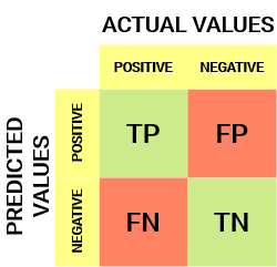
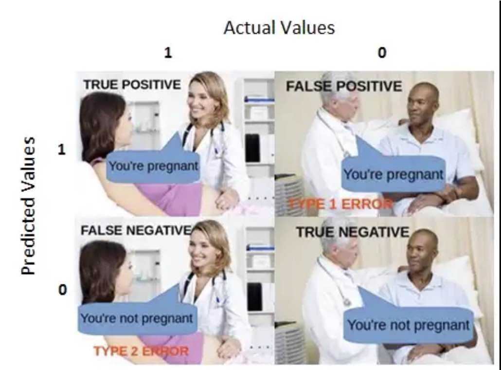
Here, TP (true positive) is the number of times the classifier predicted “positive” and the actual label was “positive”. FP (false positive) is the number of times the classifier predicted “positive” and the actual label was “negative”. FN (false negative) is the number of times the classifier predicted “negative” and the actual label was “positive”. TN (true negative) is the number of times the classifier predicted “negative” and the actual label was “negative”.
Here is an example of how to compute the values in a confusion matrix:
               Predicted
               Positive  Negative
Actual
Positive        10       5
Negative         3       2
The values in the confusion matrix can be used to compute various performance metrics, such as precision, recall, and accuracy.
Calculate Confusion Matrix for a 2 classes problem
Individual Number |
1 |
2 |
3 |
4 |
5 |
6 |
7 |
8 |
9 |
10 |
11 |
12 |
|---|---|---|---|---|---|---|---|---|---|---|---|---|
Actual Classification |
1 |
1 |
1 |
1 |
1 |
1 |
1 |
1 |
0 |
0 |
0 |
0 |
Predicted Classification |
0 |
0 |
1 |
1 |
1 |
1 |
1 |
1 |
1 |
0 |
0 |
0 |
Result |
FN |
FN |
TP |
TP |
TP |
TP |
TP |
TP |
FP |
TN |
TN |
TN |
Example from wikipedia.com
import torch
from sklearn import metrics
import matplotlib.pyplot as plt
import torchmetrics

# simulate a classification problem
y_true = torch.randint(0,2, (7,))
y_pred = torch.randint(0,2, (7,))

print(f"{y_true=}")
print(f"{y_pred=}")
print(f"confusion_matrix {metrics.confusion_matrix(y_true, y_pred)} ")

tn, fp, fn, tp = metrics.confusion_matrix(y_true, y_pred).ravel()
print(tn, fp, fn, tp)

disp = metrics.ConfusionMatrixDisplay(confusion_matrix=metrics.confusion_matrix(y_true, y_pred) )
disp.plot()
plt.show()

print(f"{torchmetrics.functional.confusion_matrix(y_true, y_pred,task='binary')=}")
y_true=tensor([1, 1, 1, 1, 1, 0, 0])
y_pred=tensor([0, 1, 1, 0, 0, 1, 0])
confusion_matrix [[1 1]
 [3 2]]
1 1 3 2

torchmetrics.functional.confusion_matrix(y_true, y_pred,task='binary')=tensor([[1, 3],
        [1, 2]])
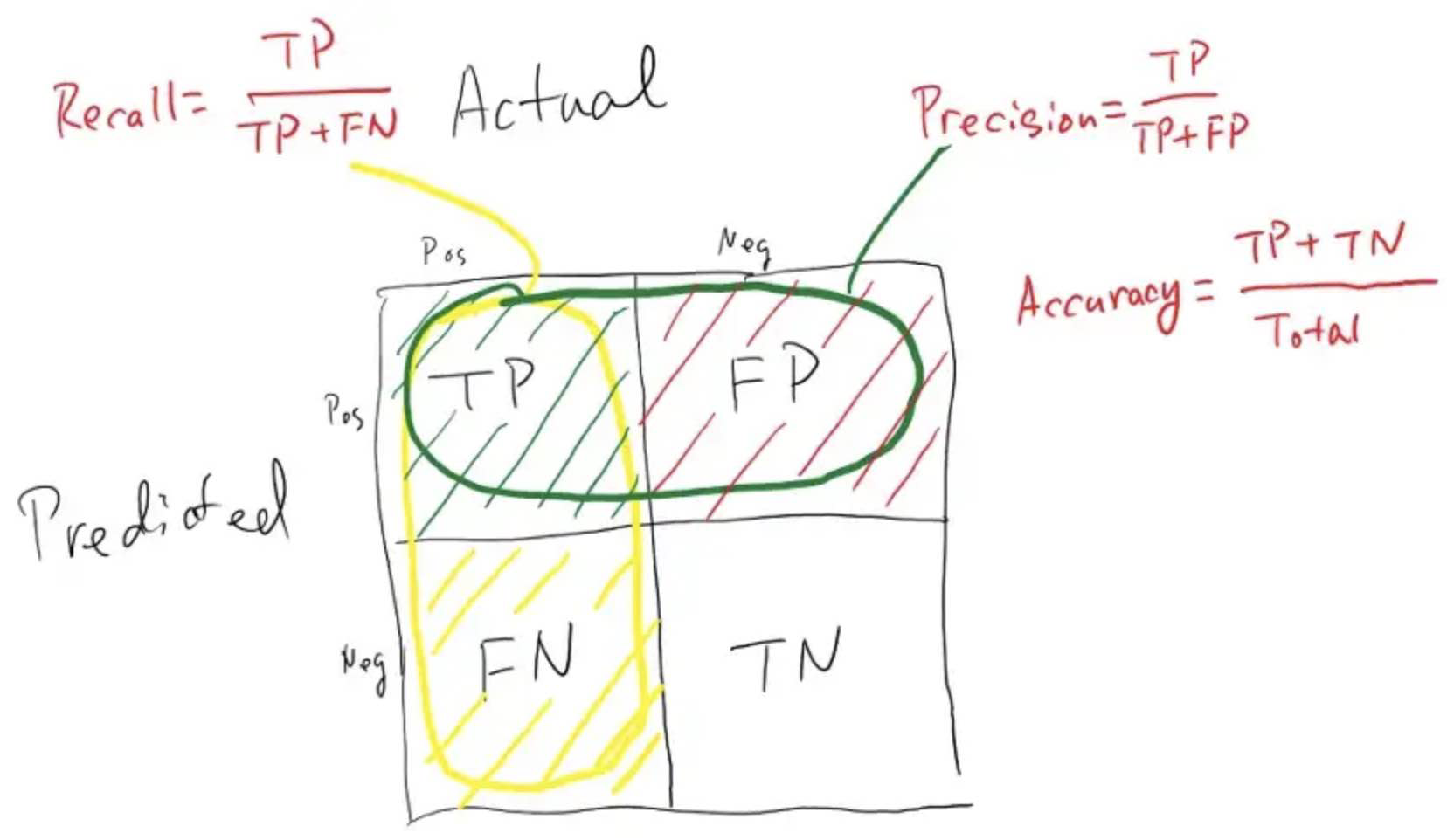
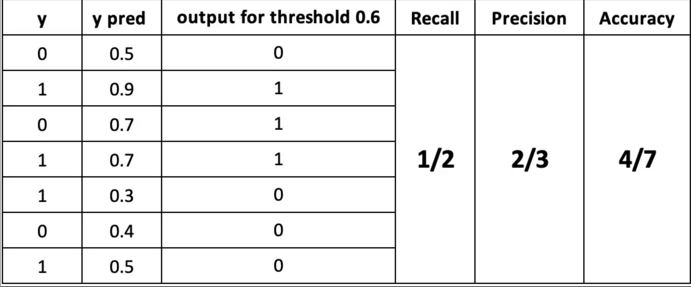
Precision
The above equation can be explained by saying, from all the classes we have predicted as positive, how many are actually positive. Precision should be high as possible.
Recall / Sensitivity / True Positive Rate
Sensitivity tells us what proportion of the positive class got correctly classified.
The above equation can be explained by saying, from all the positive classes, how many we predicted correctly. A simple example would be to determine what proportion of the actual sick people were correctly detected by the model.
Recall should be high as possible.
Note
Precision is about your prediction. Recall is about reality.
If your job is to identify thieves.
False Negative Rate
False Negative Rate (FNR) tells us what proportion of the positive class got incorrectly classified by the classifier.
A higher TPR and a lower FNR is desirable since we want to correctly classify the positive class.
Specificity / True Negative Rate
Specificity tells us what proportion of the negative class got correctly classified.
Taking the same example as in Sensitivity, Specificity would mean determining the proportion of healthy people who were correctly identified by the model.
False Positive Rate
FPR tells us what proportion of the negative class got incorrectly classified by the classifier.
A higher TNR and a lower FPR is desirable since we want to correctly classify the negative class.
Out of these metrics, Sensitivity and Specificity are perhaps the most important and we will see later on how these are used to build an evaluation metric. But before that, let’s understand why the probability of prediction is better than predicting the target class directly.
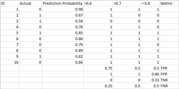
The metrics change with the changing threshold values. We can generate different confusion matrices and compare the various metrics that we discussed in the previous section. But that would not be a prudent thing to do. Instead, what we can do is generate a plot between some of these metrics so that we can easily visualize which threshold is giving us a better result.
The AUC-ROC curve solves just that problem!
print(f"{metrics.precision_score(y_true, y_pred)=}")
print(f"{metrics.recall_score(y_true, y_pred)=}")
print(f"{metrics.accuracy_score(y_true, y_pred)=}")
print(f"{metrics.f1_score(y_true, y_pred)=}")
print(f"{metrics.fbeta_score(y_true, y_pred, beta=0.5)=}")
metrics.precision_score(y_true, y_pred)=0.6666666666666666
metrics.recall_score(y_true, y_pred)=0.4
metrics.accuracy_score(y_true, y_pred)=0.42857142857142855
metrics.f1_score(y_true, y_pred)=0.5
metrics.fbeta_score(y_true, y_pred, beta=0.5)=0.5882352941176471
F1-score
The F1-score is the harmonic mean of the precision and the recall. Using the harmonic mean has the effect that a good F1-score requires both a good precision and a good recall.
It is difficult to compare two models with low precision and high recall or vice versa. So to make them comparable, we use F-Score. F-score helps to measure Recall and Precision at the same time. It uses Harmonic Mean in place of Arithmetic Mean by punishing the extreme values more.
Drawbacks
One potential drawback of the F1 score as an evaluation metric is that it is sensitive to imbalanced class distributions. This means that if one class is much more prevalent in the data than the other, the F1 score may not be a reliable indicator of the classifier’s performance.
For example, consider a binary classification problem where the positive class is rare, with only 1% of the samples belonging to that class. In this case, a classifier that simply predicts the negative class all the time would have an F1 score of 0, even though it is making the correct prediction 99% of the time. On the other hand, a classifier that makes a small number of correct predictions for the positive class (e.g., 5 out of 100) would have a relatively high F1 score, even though it is performing poorly overall.
ROC Curve and AUC
Best explaintion
https://www.analyticsvidhya.com/blog/2020/06/auc-roc-curve-machine-learning/
https://developers.google.com/machine-learning/crash-course/classification/roc-and-auc
https://stephenallwright.com/metric-choice/
https://mlu-explain.github.io/
Ranking | Recommendation | Information Retrieval
None
Language Model
ROUGE
ROUGE is actually a set of metrics that are used to evaluate the quality of a text summarization system.
ROUGE-N Overlap of n-grams[2] between the system and reference summaries.
ROUGE-1 refers to the overlap of unigram (each word) between the system and reference summaries.
ROUGE-2 refers to the overlap of bigrams between the system and reference summaries.