Derivatives and Partial Derivatives
Everything around us is changing, the universe is expanding, planets are moving, people are aging, even atoms don’t stay in the same state, they are always moving or changing. Everything is changing with time. So how do we measure it?
How things change?
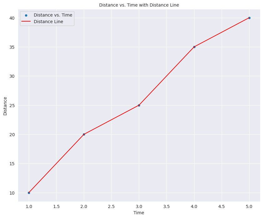
Suppose we are going on a car trip with our family. The speed of the car is constantly changing. Similarly the temperature at any given point on a day is changing. The overall temperature of Earth is changing. So we need a way to measure that change. Let’s take the example of a family trip. Suppose the overall journey of our trip looks like this:
import seaborn as sns
import matplotlib.pyplot as plt

sns.set_style('darkgrid')

params = {'legend.fontsize': 'medium',
          'figure.figsize': (10, 8),
          'figure.dpi': 100,
         'axes.labelsize': 'medium',
         'axes.titlesize':'medium',
         'xtick.labelsize':'medium',
         'ytick.labelsize':'medium'}
plt.rcParams.update(params)

# Sample data (replace this with your own data)
time = [1, 2, 3, 4, 5]
distance = [10, 20, 25, 35, 40]

# Create a scatter plot
sns.scatterplot(x=time, y=distance, label='Distance vs. Time')

# Create a line plot on top of the scatter plot
sns.lineplot(x=time, y=distance, color='red', label='Distance Line')

# Add labels and title
plt.xlabel('Time')
plt.ylabel('Distance')
plt.title('Distance vs. Time with Distance Line')

# Show legend
plt.legend()

# Show the plot
plt.show()
Average vs Instantaneous rate of change
If we look at the graph, we can see that the car covered 40 miles in 5 hours. Now the average speed or the average rate of change will be the total distance divided by total time of the whole journey which in case is
But what if we want to find the rate of change at any given time, this is where the instantaneous rate of change comes into play. The instantaneous rate of change is given by the change at any given time or point. Take the example of a speedometer which gives you the change in speed every moment. We can also calculate the instantaneous change using a graph using the concept of a slope.
Slope of a line
Slope of a line is simply defined as the rate of change in the vertical direction due to rate of change in the horizontal direction or simply
But what about the instantaneous rate of change? Well, if you look at a curved line, the slope will be different for different points.
This instantaneous rate of change at any point is called the derivative at that point and is defined as:
Derivative Explained
The derivative of a function is related to its rate of change. The rate of change tells you how much the output of the function changes when a change is done to the input. It is calculated as the ratio between a change in the output and the corresponding change in the input.
Graphically, it is the slope of the tangent at a given point of the function.
Let’s take an example. Suppose we have a function like this:
The graph of this function looks like this
# seaborn grah of x squared function
x = [-5, -4, -3, -2, -1 , 0 , 1, 2, 3, 4, 5]
func = lambda i: i**2

y = [func(i) for i in x]

sns.lineplot(x=x, y=y)
plt.show()
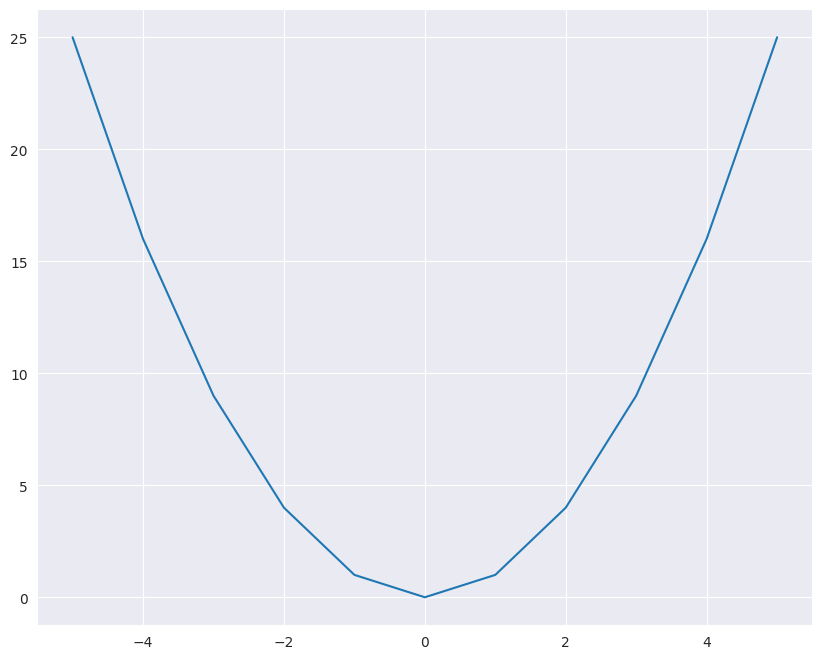
Now let’s say we want to find the slope or instantaneous change in y due to x. Let’s say x change from x to x+h then:
Lets say y changes due change in x so
then
since h -> 0 so h will be zero.
Partial Derivatives
Now considering the derivative of a function with a single input, a partial derivative of a function is just the derivative of a function with multiple inputs with respect to a single variable i.e. the change in that function caused by the change in a single input. Let’s suppose a function
Now we cannot find the derivative of this function directly since it depends on two inputs. So what we do is we find the derivative of this function assuming that one of the inputs is constant. Or simply that what change in the function is caused by the slight change in that single input. Let’s find the partial derivative of this function with respect to both inputs one by 1
To calculate the partial derivatives of the given function \((f(x, y) = x^2y + \sin(y)) \) with respect to x and y, we will find the derivative of each term separately and then combine them using the rules of partial differentiation.
Partial derivative with respect to x
denoted as \(\frac{\partial f}{\partial x}\):
We treat \(y\) as a constant when taking the derivative with respect to \(x\). Therefore, we differentiate \(x^2y\) with respect to \(x\) while keeping \(y\) constant:
The derivative of \(\sin(y)\) with respect to \(x\) is 0 because \(\sin(y)\) does not depend on \(x\). So, \(\frac{\partial}{\partial x}(\sin(y)) = 0\).
Now, we can combine these partial derivatives:
So, the partial derivative of \(f(x, y)\) with respect to \(x is \)2xy$.
Partial derivative with respect to y
denoted as \(\frac{\partial f}{\partial y}\)
Now, we treat x as a constant when taking the derivative with respect to y. Therefore, we differentiate \((x^2y\) with respect to \(y\) while keeping \(x\) constant:
The derivative of \(\sin(y)\) with respect to y is \(\cos(y)\), so \(\frac{\partial}{\partial y}(\sin(y)) = \cos(y)\).
Now, we can combine these partial derivatives:
So, the partial derivative of \(f(x, y)\) with respect to y is \(x^2 + \cos(y)\).
In summary, the partial derivatives of the given function \(f(x, y) = x^2y + \sin(y)\) are:
and
Now if we want to find the partial derivative of the function at the point (-1, 2). We can just chug in values in both partial equations and find the change as:
Similarly
So we say that the change in the function with respect to input x is -4 times and with respect to y is +0.5838.
This means that the function is more sensitive to x than to y.
E.g https://www.youtube.com/watch?v=dfvnCHqzK54
https://www.youtube.com/watch?v=wqPt3qjB6uA&ab_channel=Dr.DataScience
https://www.youtube.com/watch?v=sIX_9n-1UbM
Derivative rules
Constant Rule
If you have a number (like 5 or 10) all by itself, its derivative is always 0. This means it doesn’t change when you take the derivative.
A constant represents a horizontal line on the graph, which has no slope (i.e., it’s perfectly flat). Therefore, the rate of change (derivative) is zero.
Proof: Let \(f(x) = c\), where c is a constant. Then, by definition, the derivative of \(f(x)\) is
Power Rule
If you have a number with an exponent (like \(x^2\) or \(x^3\)), you can bring the exponent down and subtract 1 from it. For example, if you have \(x^2\), the derivative is 2x because 2 times \(x^1\) is 2x.
The derivative of \(x^n\) with respect to x is \(nx^{n-1}\), where n is a constant. This rule is derived using the limit definition of the derivative and the binomial theorem.
Proof: Start with the limit definition of the derivative
Use the binomial theorem to expand \((x+h)^n\) $\( (x+h)^n = x^n + nx^{n-1}h + \text{higher order terms in } h \)$ Substitute this into the limit definition
Cancel the \(x^n\) terms and divide by \(h\)
Simplify and take the limit as h approaches 0: $\( \frac{d}{dx}(x^n) = nx^{n-1} \)$
Sum Rule
If you’re adding or subtracting two things, like f(x) + g(x) or f(x) - g(x), you can take the derivative of each thing separately and keep them separate. For example, if you have \(3x^2 + 4x\), you can find the derivative of \(3x^2\) (which is 6x) and the derivative of 4x (which is 4), and then you keep them together as 6x + 4.
Chain Rule
Sometimes, you have functions inside of functions. Imagine you have \(f(g(x))\). To find the derivative of that, you first find the derivative of the outer function (f) and then the derivative of the inner function (g). You multiply them together. It’s like doing things step by step.
The chain rule is a fundamental rule in calculus that allows us to find the derivative of a composite function. In other words, it tells us how to differentiate a function that is composed of two or more functions. The chain rule is often stated as follows:
If f(u) and g(x) are differentiable functions, then the derivative of their composition f(g(x)) is given by:
Here’s an explanation of the chain rule with an example and a proof:
Explanation:
The chain rule essentially states that to find the derivative of a composite function, you first take the derivative of the outer function with respect to its inner function and then multiply it by the derivative of the inner function with respect to the variable of interest (in this case, x).
Example
Let’s use an example to illustrate the chain rule. Consider the function \(y = f(u) = u^2\) and \(u = g(x) = x^3\). We want to find the derivative of \(y\) with respect to \(x\) which is \(\frac{dy}{dx}\).
Find \(\frac{dy}{du}\): This is the derivative of the outer function \(f(u)\) with respect to its inner function \(u\), which is \(2u\).
Find \(\frac{du}{dx}\): This is the derivative of the inner function \(g(x)\) with respect to \(x\), which is \(3x^2\).
Apply the chain rule:
Now, substitute back \(u = x^3\):
So, the derivative of \(y = x^6\) with respect to \(x\) is \(6x^5\).
Proof:
The proof of the chain rule relies on the definition of the derivative and the limit concept. Let’s prove it step by step:
Start with the definition of the derivative of a function:
Now, we want to find the derivative of the composition \(f(g(x))\). Let \(v = g(x)\). So, we can write:
Using the definition of the derivative for \(f(v)\), we have:
Rewrite \(v + h\) as \(g(x + h)\) because \(v = g(x)\):
Now, we can see that this is precisely the definition of the derivative of \(f(g(x))\). So, we’ve shown that:
And this can be simplified to:
So, the chain rule is proven. It tells us how to find the derivative of a composite function by considering the derivatives of its components.
Backpropagation Chain rule
The chain rule is a crucial concept in neural network backpropagation, which is the algorithm used to train neural networks. It allows us to efficiently calculate the gradients of the loss function with respect to the network’s parameters (weights and biases) by decomposing the overall gradient into smaller gradients associated with each layer of the network. Let’s explain how the chain rule is used in neural network backpropagation with an example.
Suppose we have a simple feedforward neural network with one hidden layer. Here’s a simplified network architecture:
Input layer with \(n\) neurons
Hidden layer with \(m\) neurons
Output layer with \(k\) neurons
The network has weights \(W^{(1)}\) for the connections between the input and hidden layers and weights \(W^{(2)}\) for the connections between the hidden and output layers.
The forward pass of the network involves the following steps:
Compute the weighted sum and apply an activation function to the hidden layer:
where \(X\) is the input, \(W^{(1)}\) are the weights of the first layer, \(b^{(1)}\) are the biases of the first layer, \(\sigma(\cdot)\) is the activation function (e.g., sigmoid or ReLU), and \(a^{(1)}\) is the output of the hidden layer.
Compute the weighted sum and apply an activation function to the output layer:
where \(W^{(2)}\) are the weights of the second (output) layer, \(b^{(2)}\) are the biases of the second layer, and \(a^{(2)}\) is the final output of the network.
Now, let’s assume we have a loss function \(L\) that measures the error between the predicted output \(a^{(2)}\) and the true target values \(Y\). The goal of backpropagation is to update the network’s weights and biases to minimize this loss.
To do this, we need to compute the gradients of the loss with respect to the network’s parameters. The chain rule comes into play during this step. We calculate the gradients layer by layer, propagating the gradient backward through the network:
Compute the gradient of the loss with respect to the output layer’s activations: $\( \frac{\partial L}{\partial a^{(2)}} \)$
Use the chain rule to calculate the gradient of the loss with respect to the output layer’s weighted sum (\(z^{(2)}\)): $\( \frac{\partial L}{\partial z^{(2)}} = \frac{\partial L}{\partial a^{(2)}} \cdot \frac{\partial a^{(2)}}{\partial z^{(2)}} \)$
Compute the gradient of the loss with respect to the second layer’s weights and biases (\(W^{(2)}\) and \(b^{(2)}\)): $\( \frac{\partial L}{\partial W^{(2)}} = \frac{\partial L}{\partial z^{(2)}} \cdot \frac{\partial z^{(2)}}{\partial W^{(2)}} \)\( \)\( \frac{\partial L}{\partial b^{(2)}} = \frac{\partial L}{\partial z^{(2)}} \cdot \frac{\partial z^{(2)}}{\partial b^{(2)}} \)$
Use the chain rule again to calculate the gradient of the loss with respect to the hidden layer’s activations (\(a^{(1)}\)): $\( \frac{\partial L}{\partial a^{(1)}} = \frac{\partial L}{\partial z^{(2)}} \cdot \frac{\partial z^{(2)}}{\partial a^{(1)}} \)$
Compute the gradient of the loss with respect to the hidden layer’s weighted sum (\(z^{(1)}\)): $\( \frac{\partial L}{\partial z^{(1)}} = \frac{\partial L}{\partial a^{(1)}} \cdot \frac{\partial a^{(1)}}{\partial z^{(1)}} \)$
Finally, calculate the gradient of the loss with respect to the first layer’s weights and biases (\(W^{(1)}\) and \(b^{(1)}\)): $\( \frac{\partial L}{\partial W^{(1)}} = \frac{\partial L}{\partial z^{(1)}} \cdot \frac{\partial z^{(1)}}{\partial W^{(1)}} \)\( \)\( \frac{\partial L}{\partial b^{(1)}} = \frac{\partial L}{\partial z^{(1)}} \cdot \frac{\partial z^{(1)}}{\partial b^{(1)}} \)$
The chain rule allows us to compute these gradients efficiently by breaking down the overall gradient into smaller gradients associated with each layer. Once we have these gradients, we can use them to update the network’s weights and biases using optimization algorithms like gradient descent. This iterative process of forward and backward passes, driven by the chain rule, is how neural networks are trained to learn from data.
# Importing Required Libraries
from sklearn.datasets import load_iris
from sklearn.model_selection import train_test_split
import pandas as pd
import torch
import torch.nn.functional as F
import matplotlib.pyplot as plt

%matplotlib inline
#Load the dataset
data = load_iris()
data
{'data': array([[5.1, 3.5, 1.4, 0.2],
        [4.9, 3. , 1.4, 0.2],
        [4.7, 3.2, 1.3, 0.2],
        [4.6, 3.1, 1.5, 0.2],
        [5. , 3.6, 1.4, 0.2],
        [5.4, 3.9, 1.7, 0.4],
        [4.6, 3.4, 1.4, 0.3],
        [5. , 3.4, 1.5, 0.2],
        [4.4, 2.9, 1.4, 0.2],
        [4.9, 3.1, 1.5, 0.1],
        [5.4, 3.7, 1.5, 0.2],
        [4.8, 3.4, 1.6, 0.2],
        [4.8, 3. , 1.4, 0.1],
        [4.3, 3. , 1.1, 0.1],
        [5.8, 4. , 1.2, 0.2],
        [5.7, 4.4, 1.5, 0.4],
        [5.4, 3.9, 1.3, 0.4],
        [5.1, 3.5, 1.4, 0.3],
        [5.7, 3.8, 1.7, 0.3],
        [5.1, 3.8, 1.5, 0.3],
        [5.4, 3.4, 1.7, 0.2],
        [5.1, 3.7, 1.5, 0.4],
        [4.6, 3.6, 1. , 0.2],
        [5.1, 3.3, 1.7, 0.5],
        [4.8, 3.4, 1.9, 0.2],
        [5. , 3. , 1.6, 0.2],
        [5. , 3.4, 1.6, 0.4],
        [5.2, 3.5, 1.5, 0.2],
        [5.2, 3.4, 1.4, 0.2],
        [4.7, 3.2, 1.6, 0.2],
        [4.8, 3.1, 1.6, 0.2],
        [5.4, 3.4, 1.5, 0.4],
        [5.2, 4.1, 1.5, 0.1],
        [5.5, 4.2, 1.4, 0.2],
        [4.9, 3.1, 1.5, 0.2],
        [5. , 3.2, 1.2, 0.2],
        [5.5, 3.5, 1.3, 0.2],
        [4.9, 3.6, 1.4, 0.1],
        [4.4, 3. , 1.3, 0.2],
        [5.1, 3.4, 1.5, 0.2],
        [5. , 3.5, 1.3, 0.3],
        [4.5, 2.3, 1.3, 0.3],
        [4.4, 3.2, 1.3, 0.2],
        [5. , 3.5, 1.6, 0.6],
        [5.1, 3.8, 1.9, 0.4],
        [4.8, 3. , 1.4, 0.3],
        [5.1, 3.8, 1.6, 0.2],
        [4.6, 3.2, 1.4, 0.2],
        [5.3, 3.7, 1.5, 0.2],
        [5. , 3.3, 1.4, 0.2],
        [7. , 3.2, 4.7, 1.4],
        [6.4, 3.2, 4.5, 1.5],
        [6.9, 3.1, 4.9, 1.5],
        [5.5, 2.3, 4. , 1.3],
        [6.5, 2.8, 4.6, 1.5],
        [5.7, 2.8, 4.5, 1.3],
        [6.3, 3.3, 4.7, 1.6],
        [4.9, 2.4, 3.3, 1. ],
        [6.6, 2.9, 4.6, 1.3],
        [5.2, 2.7, 3.9, 1.4],
        [5. , 2. , 3.5, 1. ],
        [5.9, 3. , 4.2, 1.5],
        [6. , 2.2, 4. , 1. ],
        [6.1, 2.9, 4.7, 1.4],
        [5.6, 2.9, 3.6, 1.3],
        [6.7, 3.1, 4.4, 1.4],
        [5.6, 3. , 4.5, 1.5],
        [5.8, 2.7, 4.1, 1. ],
        [6.2, 2.2, 4.5, 1.5],
        [5.6, 2.5, 3.9, 1.1],
        [5.9, 3.2, 4.8, 1.8],
        [6.1, 2.8, 4. , 1.3],
        [6.3, 2.5, 4.9, 1.5],
        [6.1, 2.8, 4.7, 1.2],
        [6.4, 2.9, 4.3, 1.3],
        [6.6, 3. , 4.4, 1.4],
        [6.8, 2.8, 4.8, 1.4],
        [6.7, 3. , 5. , 1.7],
        [6. , 2.9, 4.5, 1.5],
        [5.7, 2.6, 3.5, 1. ],
        [5.5, 2.4, 3.8, 1.1],
        [5.5, 2.4, 3.7, 1. ],
        [5.8, 2.7, 3.9, 1.2],
        [6. , 2.7, 5.1, 1.6],
        [5.4, 3. , 4.5, 1.5],
        [6. , 3.4, 4.5, 1.6],
        [6.7, 3.1, 4.7, 1.5],
        [6.3, 2.3, 4.4, 1.3],
        [5.6, 3. , 4.1, 1.3],
        [5.5, 2.5, 4. , 1.3],
        [5.5, 2.6, 4.4, 1.2],
        [6.1, 3. , 4.6, 1.4],
        [5.8, 2.6, 4. , 1.2],
        [5. , 2.3, 3.3, 1. ],
        [5.6, 2.7, 4.2, 1.3],
        [5.7, 3. , 4.2, 1.2],
        [5.7, 2.9, 4.2, 1.3],
        [6.2, 2.9, 4.3, 1.3],
        [5.1, 2.5, 3. , 1.1],
        [5.7, 2.8, 4.1, 1.3],
        [6.3, 3.3, 6. , 2.5],
        [5.8, 2.7, 5.1, 1.9],
        [7.1, 3. , 5.9, 2.1],
        [6.3, 2.9, 5.6, 1.8],
        [6.5, 3. , 5.8, 2.2],
        [7.6, 3. , 6.6, 2.1],
        [4.9, 2.5, 4.5, 1.7],
        [7.3, 2.9, 6.3, 1.8],
        [6.7, 2.5, 5.8, 1.8],
        [7.2, 3.6, 6.1, 2.5],
        [6.5, 3.2, 5.1, 2. ],
        [6.4, 2.7, 5.3, 1.9],
        [6.8, 3. , 5.5, 2.1],
        [5.7, 2.5, 5. , 2. ],
        [5.8, 2.8, 5.1, 2.4],
        [6.4, 3.2, 5.3, 2.3],
        [6.5, 3. , 5.5, 1.8],
        [7.7, 3.8, 6.7, 2.2],
        [7.7, 2.6, 6.9, 2.3],
        [6. , 2.2, 5. , 1.5],
        [6.9, 3.2, 5.7, 2.3],
        [5.6, 2.8, 4.9, 2. ],
        [7.7, 2.8, 6.7, 2. ],
        [6.3, 2.7, 4.9, 1.8],
        [6.7, 3.3, 5.7, 2.1],
        [7.2, 3.2, 6. , 1.8],
        [6.2, 2.8, 4.8, 1.8],
        [6.1, 3. , 4.9, 1.8],
        [6.4, 2.8, 5.6, 2.1],
        [7.2, 3. , 5.8, 1.6],
        [7.4, 2.8, 6.1, 1.9],
        [7.9, 3.8, 6.4, 2. ],
        [6.4, 2.8, 5.6, 2.2],
        [6.3, 2.8, 5.1, 1.5],
        [6.1, 2.6, 5.6, 1.4],
        [7.7, 3. , 6.1, 2.3],
        [6.3, 3.4, 5.6, 2.4],
        [6.4, 3.1, 5.5, 1.8],
        [6. , 3. , 4.8, 1.8],
        [6.9, 3.1, 5.4, 2.1],
        [6.7, 3.1, 5.6, 2.4],
        [6.9, 3.1, 5.1, 2.3],
        [5.8, 2.7, 5.1, 1.9],
        [6.8, 3.2, 5.9, 2.3],
        [6.7, 3.3, 5.7, 2.5],
        [6.7, 3. , 5.2, 2.3],
        [6.3, 2.5, 5. , 1.9],
        [6.5, 3. , 5.2, 2. ],
        [6.2, 3.4, 5.4, 2.3],
        [5.9, 3. , 5.1, 1.8]]),
 'target': array([0, 0, 0, 0, 0, 0, 0, 0, 0, 0, 0, 0, 0, 0, 0, 0, 0, 0, 0, 0, 0, 0,
        0, 0, 0, 0, 0, 0, 0, 0, 0, 0, 0, 0, 0, 0, 0, 0, 0, 0, 0, 0, 0, 0,
        0, 0, 0, 0, 0, 0, 1, 1, 1, 1, 1, 1, 1, 1, 1, 1, 1, 1, 1, 1, 1, 1,
        1, 1, 1, 1, 1, 1, 1, 1, 1, 1, 1, 1, 1, 1, 1, 1, 1, 1, 1, 1, 1, 1,
        1, 1, 1, 1, 1, 1, 1, 1, 1, 1, 1, 1, 2, 2, 2, 2, 2, 2, 2, 2, 2, 2,
        2, 2, 2, 2, 2, 2, 2, 2, 2, 2, 2, 2, 2, 2, 2, 2, 2, 2, 2, 2, 2, 2,
        2, 2, 2, 2, 2, 2, 2, 2, 2, 2, 2, 2, 2, 2, 2, 2, 2, 2]),
 'frame': None,
 'target_names': array(['setosa', 'versicolor', 'virginica'], dtype='<U10'),
 'DESCR': '.. _iris_dataset:\n\nIris plants dataset\n--------------------\n\n**Data Set Characteristics:**\n\n:Number of Instances: 150 (50 in each of three classes)\n:Number of Attributes: 4 numeric, predictive attributes and the class\n:Attribute Information:\n    - sepal length in cm\n    - sepal width in cm\n    - petal length in cm\n    - petal width in cm\n    - class:\n            - Iris-Setosa\n            - Iris-Versicolour\n            - Iris-Virginica\n\n:Summary Statistics:\n\n============== ==== ==== ======= ===== ====================\n                Min  Max   Mean    SD   Class Correlation\n============== ==== ==== ======= ===== ====================\nsepal length:   4.3  7.9   5.84   0.83    0.7826\nsepal width:    2.0  4.4   3.05   0.43   -0.4194\npetal length:   1.0  6.9   3.76   1.76    0.9490  (high!)\npetal width:    0.1  2.5   1.20   0.76    0.9565  (high!)\n============== ==== ==== ======= ===== ====================\n\n:Missing Attribute Values: None\n:Class Distribution: 33.3% for each of 3 classes.\n:Creator: R.A. Fisher\n:Donor: Michael Marshall (MARSHALL%PLU@io.arc.nasa.gov)\n:Date: July, 1988\n\nThe famous Iris database, first used by Sir R.A. Fisher. The dataset is taken\nfrom Fisher\'s paper. Note that it\'s the same as in R, but not as in the UCI\nMachine Learning Repository, which has two wrong data points.\n\nThis is perhaps the best known database to be found in the\npattern recognition literature.  Fisher\'s paper is a classic in the field and\nis referenced frequently to this day.  (See Duda & Hart, for example.)  The\ndata set contains 3 classes of 50 instances each, where each class refers to a\ntype of iris plant.  One class is linearly separable from the other 2; the\nlatter are NOT linearly separable from each other.\n\n|details-start|\n**References**\n|details-split|\n\n- Fisher, R.A. "The use of multiple measurements in taxonomic problems"\n  Annual Eugenics, 7, Part II, 179-188 (1936); also in "Contributions to\n  Mathematical Statistics" (John Wiley, NY, 1950).\n- Duda, R.O., & Hart, P.E. (1973) Pattern Classification and Scene Analysis.\n  (Q327.D83) John Wiley & Sons.  ISBN 0-471-22361-1.  See page 218.\n- Dasarathy, B.V. (1980) "Nosing Around the Neighborhood: A New System\n  Structure and Classification Rule for Recognition in Partially Exposed\n  Environments".  IEEE Transactions on Pattern Analysis and Machine\n  Intelligence, Vol. PAMI-2, No. 1, 67-71.\n- Gates, G.W. (1972) "The Reduced Nearest Neighbor Rule".  IEEE Transactions\n  on Information Theory, May 1972, 431-433.\n- See also: 1988 MLC Proceedings, 54-64.  Cheeseman et al"s AUTOCLASS II\n  conceptual clustering system finds 3 classes in the data.\n- Many, many more ...\n\n|details-end|\n',
 'feature_names': ['sepal length (cm)',
  'sepal width (cm)',
  'petal length (cm)',
  'petal width (cm)'],
 'filename': 'iris.csv',
 'data_module': 'sklearn.datasets.data'}
# Making it a 2 class problem
X_data = data["data"][:100]
Y_data = data["target"][:100]
len(X_data)
100
# Splitting the data into training and testing with 80 and 20%
X_train, X_test, Y_train, Y_test = train_test_split(X_data, Y_data, test_size = 0.2)
print(X_train.shape, X_test.shape)
(80, 4) (20, 4)
# Making their tensors
X_train_tensor = torch.tensor(X_train, dtype=torch.float32).t()
Y_train_tensor = torch.tensor(Y_train, dtype=torch.float32)
X_test_tensor = torch.tensor(X_test, dtype=torch.float32).t()
Y_test_tensor = torch.tensor(Y_test, dtype=torch.float32)
X_train_tensor.shape[1]
80
def init_params(n_x, n_h, n_y):
  '''
    This function is used to initializw the weights for the NN.
    n_x : input units
    n_h : hidden units
    n_y : output units
    It returns a dictionary which contains all the parameters
  '''
  W1 = torch.rand(n_x, n_h)
  b1 = torch.rand(n_h, 1)
  W2 = torch.rand(n_y, n_h)
  b2 = torch.rand(n_y, 1)

  params = {
      'W1': W1,
      'b1': b1,
      'W2': W2,
      'b2': b2
  }
  return params

def compute_cost(y_pred, y_actual):
  '''
    Uses the binary cross entropy loss to compute the cost
  '''
  return -(y_pred.log()* y_actual + (1-y_actual)*(1-y_pred).log()).mean()
  return -1/len(y_pred) * (y_actual * torch.log(y_pred) + (1 - y_actual) * torch.log(1 - y_pred)).sum()

def forward_propagation(params, x_input):
  '''
    Performs the forward propagation step. Uses the parameters to predict the output A2
  '''
  #Extractng the parameters
  W1 = params['W1']
  b1 = params['b1']
  W2 = params['W2']
  b2 = params['b2']

  # Computing the first layer
  Z1 = torch.mm(W1.t(), x_input) + b1
  A1 = torch.sigmoid(Z1)

  # Computing the second layer
  Z2 = torch.mm(W2, A1) + b2
  A2 = torch.sigmoid(Z2)

  # Returning the data
  data = {
      'Z1' : Z1,
      'A1' : A1,
      'Z2' : Z2,
      'A2' : A2
  }

  return A2, data

def back_propagation(params, data, x_input, y_input, learning_rate):
  '''
    Performs the back propagation step. Computes the gradients and updates the parameters
  '''
  m = x_input.shape[1]

  # Extracting the parameters
  W1 = params['W1']
  W2 = params['W2']
  b1 = params['b1']
  b2 = params['b2']

  # Extrcting the required predictions of first and second layers
  A1 = data['A1']
  A2 = data['A2']

  # Calculating the Gradients
  dZ2 = A2 - y_input
  dW2 = 1/m*(torch.mm(dZ2, A1.t()))
  db2 = 1/m*(torch.sum(dZ2, keepdims=True, axis=1))
  dZ1 = torch.mm(W2.t(), dZ2)*(1-torch.pow(A1,2))
  dW1 = 1/m*(torch.mm(dZ1, x_input.t()))
  db1 = 1/m*(torch.sum(dZ1, keepdims=True, axis=1))

  # Updating the parameters
  W1 -= learning_rate*dW1
  W2 -= learning_rate*dW2
  b1 -= learning_rate*db1
  b2 -= learning_rate*db2

  parameters = {"W1": W1,
                  "b1": b1,
                  "W2": W2,
                  "b2": b2}

  return parameters
def model(x_input, y_input, learning_rate = 0.01, no_iterations = 20000):
  '''
    Putting everything together and making the model
  '''
  n_x = x_input.shape[0]
  n_h = 4
  n_y = 1
  parameters = init_params(n_x, n_h, n_y)
  costs, iterations = [], []
  for i in range(no_iterations):
    A2, data = forward_propagation(parameters, x_input)

    cost = compute_cost(A2, y_input)
    cost_torch = F.binary_cross_entropy(A2, y_input.view(1, 80))

    parameters = back_propagation(parameters, data, x_input, y_input, learning_rate)

    if i%(no_iterations/20) == 0:
      print(f'Cost at iteration {i} is {cost}')
      print(f'Cost_torch at iteration {i} is {cost_torch.item()}')

    costs.append(cost)
    iterations.append(i)
  return parameters, costs, iterations
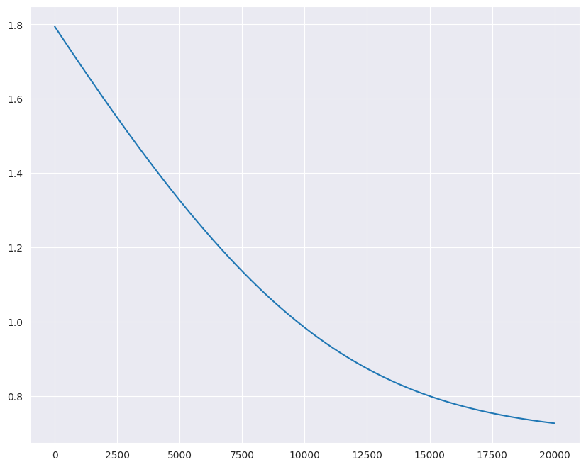
parameters, costs, iterations = model(X_train_tensor, Y_train_tensor, 1e-4, 20000)
plt.plot(iterations, costs)
Cost at iteration 0 is 1.7942848205566406
Cost_torch at iteration 0 is 1.7942848205566406
Cost at iteration 1000 is 1.6939868927001953
Cost_torch at iteration 1000 is 1.6939868927001953
Cost at iteration 2000 is 1.5964847803115845
Cost_torch at iteration 2000 is 1.5964847803115845
Cost at iteration 3000 is 1.5023094415664673
Cost_torch at iteration 3000 is 1.5023094415664673
Cost at iteration 4000 is 1.4120407104492188
Cost_torch at iteration 4000 is 1.4120407104492188
Cost at iteration 5000 is 1.3262826204299927
Cost_torch at iteration 5000 is 1.3262826204299927
Cost at iteration 6000 is 1.2456367015838623
Cost_torch at iteration 6000 is 1.2456367015838623
Cost at iteration 7000 is 1.1706621646881104
Cost_torch at iteration 7000 is 1.1706621646881104
Cost at iteration 8000 is 1.1018321514129639
Cost_torch at iteration 8000 is 1.1018321514129639
Cost at iteration 9000 is 1.0394909381866455
Cost_torch at iteration 9000 is 1.0394909381866455
Cost at iteration 10000 is 0.9838181734085083
Cost_torch at iteration 10000 is 0.9838181734085083
Cost at iteration 11000 is 0.9348093867301941
Cost_torch at iteration 11000 is 0.9348095059394836
Cost at iteration 12000 is 0.8922765851020813
Cost_torch at iteration 12000 is 0.8922765851020813
Cost at iteration 13000 is 0.8558667898178101
Cost_torch at iteration 13000 is 0.8558667898178101
Cost at iteration 14000 is 0.825097918510437
Cost_torch at iteration 14000 is 0.8250978589057922
Cost at iteration 15000 is 0.7994016408920288
Cost_torch at iteration 15000 is 0.7994016408920288
Cost at iteration 16000 is 0.7781685590744019
Cost_torch at iteration 16000 is 0.7781685590744019
Cost at iteration 17000 is 0.7607866525650024
Cost_torch at iteration 17000 is 0.7607866525650024
Cost at iteration 18000 is 0.7466720342636108
Cost_torch at iteration 18000 is 0.7466720342636108
Cost at iteration 19000 is 0.7352896928787231
Cost_torch at iteration 19000 is 0.7352896928787231
[<matplotlib.lines.Line2D at 0x7f6519d8c250>]