Graphs Data Structure

Binary Search Tree

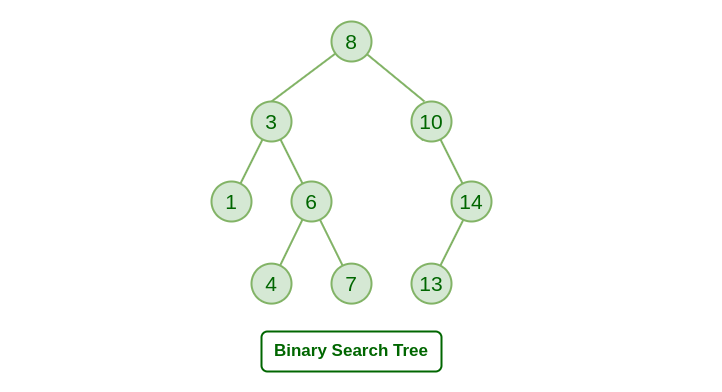
A Binary Search Tree (BST) is a special type of binary tree in which the left child of a node has a value less than the node’s value and the right child has a value greater than the node’s value. This property is called the BST property and it makes it possible to efficiently search, insert, and delete elements in the tree.

In a Binary search tree, the value of left node must be smaller than the parent node, and the value of right node must be greater than the parent node. This rule is applied recursively to the left and right subtrees of the root.

Left node > Parent node > Right node

Advantages of Binary search tree

Searching an element in the Binary search tree is easy as we always have a hint that which subtree has the desired element.

As compared to array and linked lists, insertion and deletion operations are faster in BST.

class Node: 
    # Implement a node of the binary search tree.
    # Constructor for a node with key and a given parent
    # parent can be None for a root node.
    def __init__(self, key, parent = None): 
        self.key = key
        self.parent = parent 
        self.left = None # We will set left and right child to None
        self.right = None
        # Make sure that the parent's left/right pointer
        # will point to the newly created node.
        if parent != None:
            if key < parent.key:
                assert(parent.left == None), 'parent already has a left child -- unable to create node'
                parent.left = self
            else: 
                assert key > parent.key, 'key is same as parent.key. We do not allow duplicate keys in a BST since it breaks some of the algorithms.'
                assert(parent.right == None ), 'parent already has a right child -- unable to create node'
                parent.right = self
        
    # Utility function that keeps traversing left until it finds 
    # the leftmost descendant
    def get_leftmost_descendant(self):
        if self.left != None:
            return self.left.get_leftmost_descendant()
        else:
            return self
    

    # You can call search recursively on left or right child
    # as appropriate.
    # If search succeeds: return a tuple True and the node in the tree
    # with the key we are searching for.
    # Also note that if the search fails to find the key 
    # you should return a tuple False and the node which would
    # be the parent if we were to insert the key subsequently.
    def search(self, key):
        if self.key == key: 
            return (True, self)
        # your code here
        if self.key < key and self.right != None:
            return self.right.search(key)

        if self.key > key and self.left != None:
            return self.left.search(key)
        
        return (False, self)
        
        
        
    # To insert first search for it and find out
    # the parent whose child the currently inserted key will be.
    # Create a new node with that key and insert.
    # return None if key already exists in the tree.
    # return the new node corresponding to the inserted key otherwise.
    def insert(self, key):
        # your code here
        (b, found_node) = self.search(key)
        if b is not False:
            return None
        else:
            return Node(key, found_node)
        
        
    # height of a node whose children are both None is defined
    # to be 1.
    # height of any other node is 1 + maximum of the height 
    # of its children.
    # Return a number that is th eheight.
    def height(self):
        # your code here
        if self.left is None and self.right is None:
            return 1
        elif self.left is None:
            return 1 + self.right.height()
        elif self.right is None:
            return 1 + self.left.height()
        else:
            return 1 + max(self.left.height(), self.right.height())
        
    
    # programming.
    # Case 1: both children of the node are None
    #   -- in this case, deletion is easy: simply find out if the node with key is its
    #      parent's left/right child and set the corr. child to None in the parent node.
    # Case 2: one of the child is None and the other is not.
    #   -- replace the node with its only child. In other words,
    #      modify the parent of the child to be the to be deleted node's parent.
    #      also change the parent's left/right child appropriately.
    # Case 3: both children of the parent are not None.
    #    -- first find its successor (go one step right and all the way to the left).
    #    -- function get_leftmost_descendant may be helpful here.
    #    -- replace the key of the node by its successor.
    #    -- delete the successor node.
    # return: no return value specified
    
    def delete(self, key):
        (found, node_to_delete) = self.search(key)
        assert(found == True), f"key to be deleted:{key}- does not exist in the tree"
        # your code here
        if node_to_delete.left is None and node_to_delete.right is None:
            if node_to_delete.parent.left == node_to_delete:
                node_to_delete.parent.left = None
            else:
                node_to_delete.parent.right = None
        elif node_to_delete.left is None:
            if node_to_delete.parent.left == node_to_delete:
                node_to_delete.parent.left = node_to_delete.right
            else:
                node_to_delete.parent.right = node_to_delete.right
        elif node_to_delete.right is None:
            if node_to_delete.parent.left == node_to_delete:
                node_to_delete.parent.left = node_to_delete.left
            else:
                node_to_delete.parent.right = node_to_delete.left
        else:
            successor = node_to_delete.right.get_leftmost_descendant()
            node_to_delete.key = successor.key
            successor.delete(successor.key)

t1 = Node(25, None)
t2 = Node(12, t1)
t3 = Node(18, t2)
t4 = Node(40, t1)

print('-- Testing basic node construction (originally provided code) -- ')
assert(t1.left == t2), 'test 1 failed'
assert(t2.parent == t1),  'test 2 failed'
assert(t2.right == t3), 'test 3 failed'
assert (t3.parent == t2), 'test 4 failed'
assert(t1.right == t4), 'test 5 failed'
assert(t4.left == None), 'test 6 failed'
assert(t4.right == None), 'test 7 failed'
# The tree should be : 
#             25
#             /\
#         12     40
#         /\
#     None  18
#

print('-- Testing search -- ')
(b, found_node) = t1.search(18)
assert b and found_node.key == 18, 'test 8 failed'
(b, found_node) = t1.search(25)
assert b and found_node.key == 25, 'test 9 failed -- you should find the node with key 25 which is the root'
(b, found_node) = t1.search(26)
assert(not b), 'test 10 failed'
assert(found_node.key == 40), 'test 11 failed -- you should be returning the leaf node which would be the parent to the node you failed to find if it were to be inserted in the tree.'

print('-- Testing insert -- ')
ins_node = t1.insert(26)
assert ins_node.key == 26, ' test 12 failed '
assert ins_node.parent == t4,  ' test 13 failed '
assert t4.left == ins_node,  ' test 14 failed '

ins_node2 = t1.insert(33)
assert ins_node2.key == 33, 'test 15 failed'
assert ins_node2.parent == ins_node, 'test 16 failed'
assert ins_node.right == ins_node2, 'test 17 failed'

print('-- Testing height -- ')

assert t1.height() == 4, 'test 18 failed'
assert t4.height() == 3, 'test 19 failed'
assert t2.height() == 2, 'test 20 failed'


# Testing deletion
t1 = Node(16, None)
# insert the nodes in the list
lst = [18,25,10, 14, 8, 22, 17, 12]
for elt in lst:
    t1.insert(elt)

# The tree should look like this
#               16
#            /     \
#          10      18
#        /  \     /  \
#       8   14   17  25
#          /         /  
#         12        22


# Let us test the three deletion cases.
# case 1 let's delete node 8
# node 8 does not have left or right children.
t1.delete(8) # should have both children nil.
(b8,n8) = t1.search(8)
assert not b8, 'Test A: deletion fails to delete node.'
(b,n) = t1.search(10)
assert( b) , 'Test B failed: search does not work'
assert n.left == None, 'Test C failed: Node 8 was not properly deleted.'

# Let us test deleting the node 14 whose right child is none.
# n is still pointing to the node 10 after deleting 8.
# let us ensure that it's right child is 14
assert n.right != None, 'Test D failed: node 10 should have right child 14'
assert n.right.key == 14, 'Test E failed: node 10 should have right child 14'

# Let's delete node 14
t1.delete(14)
(b14, n14) = t1.search(14)
assert not b14, 'Test F: Deletion of node 14 failed -- it still exists in the tree.'
(b,n) = t1.search(10)
assert n.right != None , 'Test G failed: deletion of node 14 not handled correctly'
assert n.right.key == 12, f'Test H failed: deletion of node 14 not handled correctly: {n.right.key}'

# Let's delete node 18 in the tree. 
# It should be replaced by 22.

t1.delete(18)
(b18, n18) = t1.search(18)
assert not b18, 'Test I: Deletion of node 18 failed'
assert t1.right.key == 22 , ' Test J: Replacement of node with successor failed.'
assert t1.right.right.left == None, ' Test K: replacement of node with successor failed -- you did not delete the successor leaf properly?'

-- Testing basic node construction (originally provided code) -- 
-- Testing search -- 
-- Testing insert -- 
-- Testing height -- 

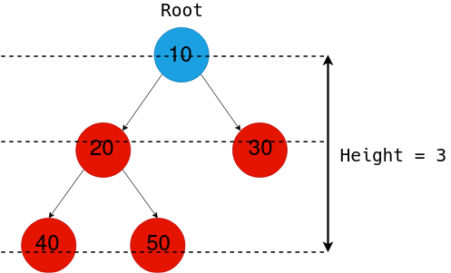
Height of BST

The height of a Binary Tree is defined as the maximum depth of any leaf node from the root node. That is, it is the length of the longest path from the root node to any leaf node.

Find in BST

Complexity: O(log n) and O(n) in worst case

Insertion and Deleteion in BST

class Node:
    def __init__(self, key):
        self.left = None
        self.right = None
        self.val = key

def insert(root, key):
    if root is None:
        return Node(key)
    else:
        if root.val == key:
            return root
        elif root.val < key:
            root.right = insert(root.right, key)
        else:
            root.left = insert(root.left, key)
    return root

def inorder(root):
    if root:
        inorder(root.left)
        print(root.val, end =" ")
        inorder(root.right)


if __name__ == '__main__':

    # Let us create the following BST
    # 50
    #  /     \
    # 30     70
    #  / \ / \
    # 20 40 60 80

    r = Node(50)
    r = insert(r, 30)
    r = insert(r, 20)
    r = insert(r, 40)
    r = insert(r, 70)
    r = insert(r, 60)
    r = insert(r, 80)

    # Print inorder traversal of the BST
    inorder(r)

20 30 40 50 60 70 80

Delete a node from BST

# Python program to demonstrate delete operation
# in binary search tree

# A Binary Tree Node


class Node:

	# Constructor to create a new node
	def __init__(self, key):
		self.key = key
		self.left = None
		self.right = None


# A utility function to do inorder traversal of BST
def inorder(root):
	if root is not None:
		inorder(root.left)
		print(root.key, end=" ")
		inorder(root.right)


# A utility function to insert a
# new node with given key in BST
def insert(node, key):

	# If the tree is empty, return a new node
	if node is None:
		return Node(key)

	# Otherwise recur down the tree
	if key < node.key:
		node.left = insert(node.left, key)
	else:
		node.right = insert(node.right, key)

	# return the (unchanged) node pointer
	return node

# Given a non-empty binary
# search tree, return the node
# with minimum key value
# found in that tree. Note that the
# entire tree does not need to be searched


def minValueNode(node):
	current = node

	# loop down to find the leftmost leaf
	while(current.left is not None):
		current = current.left

	return current

# Given a binary search tree and a key, this function
# delete the key and returns the new root


def deleteNode(root, key):

	# Base Case
	if root is None:
		return root

	# If the key to be deleted
	# is smaller than the root's
	# key then it lies in left subtree
	if key < root.key:
		root.left = deleteNode(root.left, key)

	# If the kye to be delete
	# is greater than the root's key
	# then it lies in right subtree
	elif(key > root.key):
		root.right = deleteNode(root.right, key)

	# If key is same as root's key, then this is the node
	# to be deleted
	else:

		# Node with only one child or no child
		if root.left is None:
			temp = root.right
			root = None
			return temp

		elif root.right is None:
			temp = root.left
			root = None
			return temp

		# Node with two children:
		# Get the inorder successor
		# (smallest in the right subtree)
		temp = minValueNode(root.right)

		# Copy the inorder successor's
		# content to this node
		root.key = temp.key

		# Delete the inorder successor
		root.right = deleteNode(root.right, temp.key)

	return root


# Driver code
""" Let us create following BST
			50
		/	 \
		30	 70
		/ \ / \
	20 40 60 80 """

root = None
root = insert(root, 50)
root = insert(root, 30)
root = insert(root, 20)
root = insert(root, 40)
root = insert(root, 70)
root = insert(root, 60)
root = insert(root, 80)

print("Inorder traversal of the given tree")
inorder(root)

print("\nDelete 20")
root = deleteNode(root, 20)
print("Inorder traversal of the modified tree")
inorder(root)

print("\nDelete 30")
root = deleteNode(root, 30)
print("Inorder traversal of the modified tree")
inorder(root)

print("\nDelete 50")
root = deleteNode(root, 50)
print("Inorder traversal of the modified tree")
inorder(root)

# This code is contributed by Nikhil Kumar Singh(nickzuck_007)

Inorder traversal of the given tree
20 30 40 50 60 70 80 
Delete 20
Inorder traversal of the modified tree
30 40 50 60 70 80 
Delete 30
Inorder traversal of the modified tree
40 50 60 70 80 
Delete 50
Inorder traversal of the modified tree
40 60 70 80 

Traversals – Inorder, Preorder, Post Order

Given a Binary Search Tree, The task is to print the elements in inorder, preorder, and postorder traversal of the Binary Search Tree.

Inorder Traversal: 10 20 30 100 150 200 300

Preorder Traversal: 100 20 10 30 200 150 300

Postorder Traversal: 10 30 20 150 300 200 100

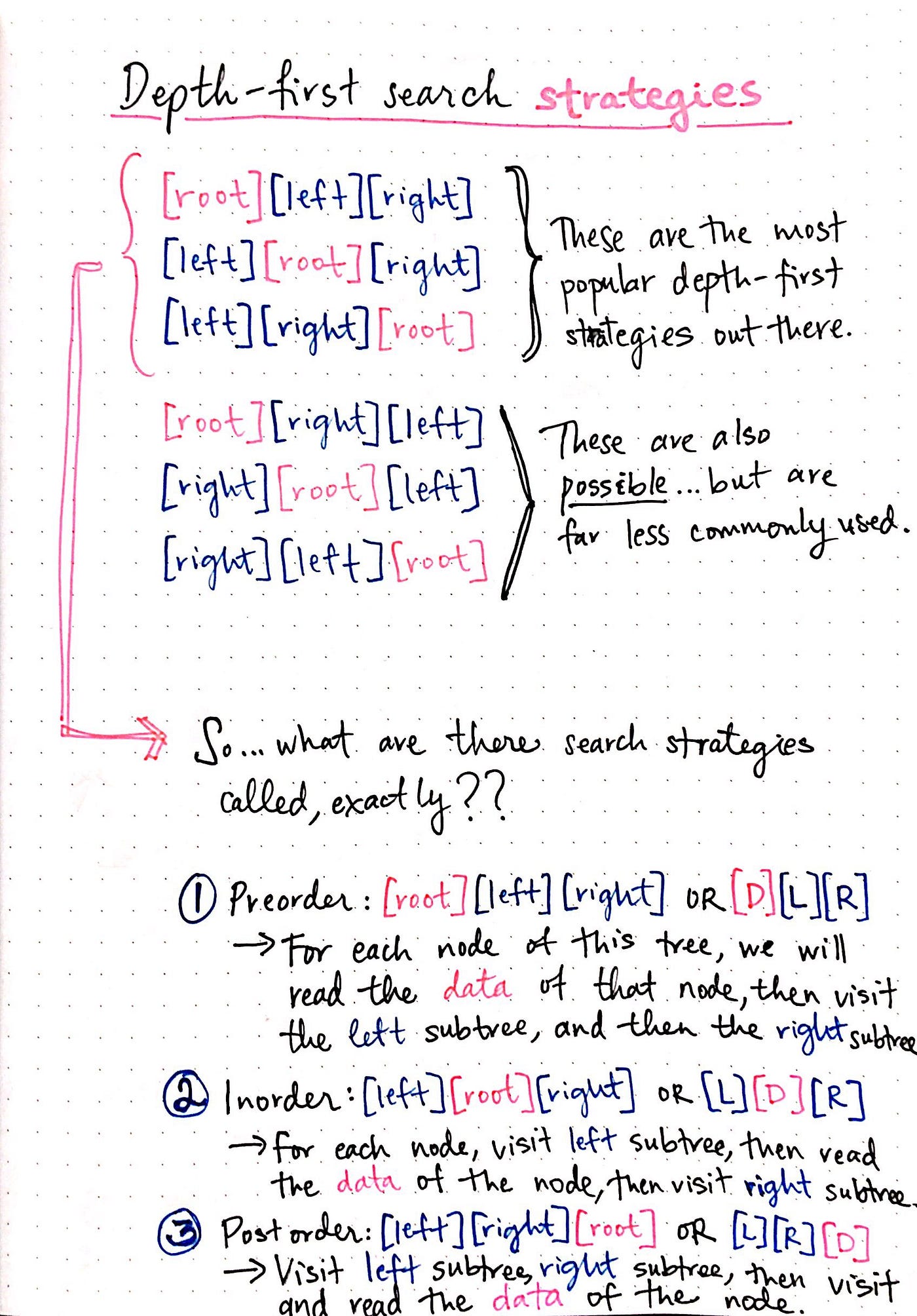
Inorder Traversal:

Traverse left subtree Visit the root and print the data. Traverse the right subtree

class Node:
	def __init__(self, v):
		self.left = None
		self.right = None
		self.data = v

# Inorder Traversal
def printInorder(root):
	if root:
		# Traverse left subtree
		printInorder(root.left)
		
		# Visit node
		print(root.data,end=" ")
		
		# Traverse right subtree
		printInorder(root.right)

# Driver code
if __name__ == "__main__":
	# Build the tree
	root = Node(100)
	root.left = Node(20)
	root.right = Node(200)
	root.left.left = Node(10)
	root.left.right = Node(30)
	root.right.left = Node(150)
	root.right.right = Node(300)

	# Function call
	print("Inorder Traversal:",end=" ")
	printInorder(root)

	# This code is contributed by ajaymakvana.

Inorder Traversal: 10 20 30 100 150 200 300

Preorder Traversal

At first visit the root then traverse left subtree and then traverse the right subtree.

Follow the below steps to implement the idea:

Visit the root and print the data.
Traverse left subtree
Traverse the right subtree

class Node:
	def __init__(self, v):
		self.data = v
		self.left = None
		self.right = None

# Preorder Traversal
def printPreOrder(node):
	if node is None:
		return
	# Visit Node
	print(node.data, end = " ")

	# Traverse left subtree
	printPreOrder(node.left)

	# Traverse right subtree
	printPreOrder(node.right)

# Driver code
if __name__ == "__main__":
	# Build the tree
	root = Node(100)
	root.left = Node(20)
	root.right = Node(200)
	root.left.left = Node(10)
	root.left.right = Node(30)
	root.right.left = Node(150)
	root.right.right = Node(300)

	# Function call
	print("Preorder Traversal: ", end = "")
	printPreOrder(root)

Preorder Traversal: 100 20 10 30 200 150 300

Postorder Traversal

At first traverse left subtree then traverse the right subtree and then visit the root.

Follow the below steps to implement the idea:

Traverse left subtree
Traverse the right subtree
Visit the root and print the data.

class Node:
	def __init__(self, v):
		self.data = v
		self.left = None
		self.right = None

# Preorder Traversal
def printPostOrder(node):
	if node is None:
		return

	# Traverse left subtree
	printPostOrder(node.left)

	# Traverse right subtree
	printPostOrder(node.right)
	
	# Visit Node
	print(node.data, end = " ")

# Driver code
if __name__ == "__main__":
	# Build the tree
	root = Node(100)
	root.left = Node(20)
	root.right = Node(200)
	root.left.left = Node(10)
	root.left.right = Node(30)
	root.right.left = Node(150)
	root.right.right = Node(300)

	# Function call
	print("Postorder Traversal: ", end = "")
	printPostOrder(root)

Postorder Traversal: 10 30 20 150 300 200 100

Red-Black Tree

When it comes to searching and sorting data, one of the most fundamental data structures is the binary search tree. However, the performance of a binary search tree is highly dependent on its shape, and in the worst case, it can degenerate into a linear structure with a time complexity of O(n). This is where Red Black Trees come in, they are a type of balanced binary search tree that use a specific set of rules to ensure that the tree is always balanced. This balance guarantees that the time complexity for operations such as insertion, deletion, and searching is always O(log n), regardless of the initial shape of the tree.

Red Black Trees are self-balancing, meaning that the tree adjusts itself automatically after each insertion or deletion operation. It uses a simple but powerful mechanism to maintain balance, by coloring each node in the tree either red or black.

Properties of Red Black Tree

The Red-Black tree satisfies all the properties of binary search tree in addition to that it satisfies following additional properties –

Root property: The root is black.
External property: Every leaf (Leaf is a NULL child of a node) is black in Red-Black tree.
Internal property: The children of a red node are black. Hence possible parent of red node is a black node.
Depth property: All the leaves have the same black depth.
Path property: Every simple path from root to descendant leaf node contains same number of black nodes.

The result of all these above-mentioned properties is that the Red-Black tree is roughly balanced.

Graph Data Structure

A graph is a non-linear data structure consisting of nodes and edges. The nodes are sometimes also referred to as vertices and the edges are lines or arcs that connect any two nodes in the graph. More formally a Graph can be defined as, a Graph consists of a finite set of vertices(or nodes) and set of Edges which connect a pair of nodes.

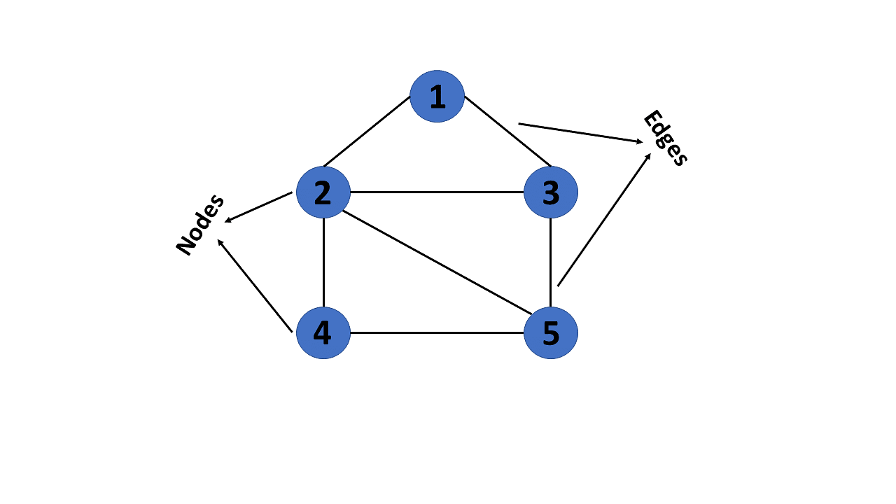
In graph theory, a graph is a mathematical structure consisting of a set of objects, called vertices or nodes, and a set of connections, called edges, which link pairs of vertices. The notation:

\[ G = (V, E) \]

is used to represent a graph, where \(G\) is the graph, \(V\) is the set of vertices, and \(\bigvee\) is the set of edges.

The nodes of a graph can represent any objects, such as cities, people, web pages, or molecules, and the edges represent the relationships or connections between them.

import networkx as nx
import matplotlib.pyplot as plt

G = nx.Graph()
G.add_edges_from([('A', 'B'), ('A', 'C'), ('B', 'D'), ('B', 'E'), ('C', 'F'), ('C', 'G')])

plt.axis('off')
nx.draw_networkx(G,
                 pos=nx.spring_layout(G, seed=0),
                 node_size=600,
                 cmap='coolwarm',
                 font_size=14,
                 font_color='white'
                 )

Matplotlib is building the font cache; this may take a moment.

---------------------------------------------------------------------------
KeyboardInterrupt                         Traceback (most recent call last)
Cell In[7], line 2
      1 import networkx as nx
----> 2 import matplotlib.pyplot as plt
      4 G = nx.Graph()
      5 G.add_edges_from([('A', 'B'), ('A', 'C'), ('B', 'D'), ('B', 'E'), ('C', 'F'), ('C', 'G')])

File ~/checkouts/readthedocs.org/user_builds/ml-math/envs/latest/lib/python3.11/site-packages/matplotlib/pyplot.py:56
     54 from cycler import cycler
     55 import matplotlib
---> 56 import matplotlib.colorbar
     57 import matplotlib.image
     58 from matplotlib import _api

File ~/checkouts/readthedocs.org/user_builds/ml-math/envs/latest/lib/python3.11/site-packages/matplotlib/colorbar.py:19
     16 import numpy as np
     18 import matplotlib as mpl
---> 19 from matplotlib import _api, cbook, collections, cm, colors, contour, ticker
     20 import matplotlib.artist as martist
     21 import matplotlib.patches as mpatches

File ~/checkouts/readthedocs.org/user_builds/ml-math/envs/latest/lib/python3.11/site-packages/matplotlib/contour.py:15
     13 import matplotlib as mpl
     14 from matplotlib import _api, _docstring
---> 15 from matplotlib.backend_bases import MouseButton
     16 from matplotlib.lines import Line2D
     17 from matplotlib.path import Path

File ~/checkouts/readthedocs.org/user_builds/ml-math/envs/latest/lib/python3.11/site-packages/matplotlib/backend_bases.py:46
     43 import numpy as np
     45 import matplotlib as mpl
---> 46 from matplotlib import (
     47     _api, backend_tools as tools, cbook, colors, _docstring, text,
     48     _tight_bbox, transforms, widgets, is_interactive, rcParams)
     49 from matplotlib._pylab_helpers import Gcf
     50 from matplotlib.backend_managers import ToolManager

File ~/checkouts/readthedocs.org/user_builds/ml-math/envs/latest/lib/python3.11/site-packages/matplotlib/text.py:16
     14 from . import _api, artist, cbook, _docstring
     15 from .artist import Artist
---> 16 from .font_manager import FontProperties
     17 from .patches import FancyArrowPatch, FancyBboxPatch, Rectangle
     18 from .textpath import TextPath, TextToPath  # noqa # Logically located here

File ~/checkouts/readthedocs.org/user_builds/ml-math/envs/latest/lib/python3.11/site-packages/matplotlib/font_manager.py:1582
   1578     _log.info("generated new fontManager")
   1579     return fm
-> 1582 fontManager = _load_fontmanager()
   1583 findfont = fontManager.findfont
   1584 get_font_names = fontManager.get_font_names

File ~/checkouts/readthedocs.org/user_builds/ml-math/envs/latest/lib/python3.11/site-packages/matplotlib/font_manager.py:1576, in _load_fontmanager(try_read_cache)
   1574             _log.debug("Using fontManager instance from %s", fm_path)
   1575             return fm
-> 1576 fm = FontManager()
   1577 json_dump(fm, fm_path)
   1578 _log.info("generated new fontManager")

File ~/checkouts/readthedocs.org/user_builds/ml-math/envs/latest/lib/python3.11/site-packages/matplotlib/font_manager.py:1043, in FontManager.__init__(self, size, weight)
   1040 for path in [*findSystemFonts(paths, fontext=fontext),
   1041              *findSystemFonts(fontext=fontext)]:
   1042     try:
-> 1043         self.addfont(path)
   1044     except OSError as exc:
   1045         _log.info("Failed to open font file %s: %s", path, exc)

File ~/checkouts/readthedocs.org/user_builds/ml-math/envs/latest/lib/python3.11/site-packages/matplotlib/font_manager.py:1076, in FontManager.addfont(self, path)
   1074     self.afmlist.append(prop)
   1075 else:
-> 1076     font = ft2font.FT2Font(path)
   1077     prop = ttfFontProperty(font)
   1078     self.ttflist.append(prop)

KeyboardInterrupt: 

Terminology

The following are the most commonly used terms in graph theory with respect to graphs:

Vertex - A vertex, also called a “node”, is a fundamental part of a graph. In the context of graphs, a vertex is an object which may contain zero or more items called attributes.
Edge - An edge is a connection between two vertices. An edge may contain a weight/value/cost.
Path - A path is a sequence of edges connecting a sequence of vertices.
Cycle - A cycle is a path of edges that starts and ends on the same vertex.
Weighted Graph/Network - A weighted graph is a graph with numbers assigned to its edges. These numbers are called weights.
Unweighted Graph/Network - An unweighted graph is a graph in which all edges have equal weight.
Directed Graph/Network - A directed graph is a graph where all the edges are directed.
Undirected Graph/Network - An undirected graph is a graph where all the edges are not directed.
Adjacent Vertices - Two vertices in a graph are said to be adjacent if there is an edge connecting them.

Types of Graphs

There are two types of graphs:

Directed Graphs
Undirected Graphs
Weighted Graph
Cyclic Graph
Acyclic Graph
Directed Acyclic Graph

Directed Graphs

In a directed graph, all the edges are directed. That means, each edge is associated with a direction. For example, if there is an edge from node A to node B, then the edge is directed from A to B and not the other way around.

Directed graph, also called a digraph.

DG = nx.DiGraph()
DG.add_edges_from([('A', 'B'), ('A', 'C'), ('B', 'D'),  
('B', 'E'), ('C', 'F'), ('C', 'G')])
nx.draw_networkx(DG, pos=nx.spring_layout(DG, seed=0), node_size=600, cmap='coolwarm', font_size=14, font_color='white')

Undirected Graphs

In an undirected graph, all the edges are undirected. That means, each edge is associated with a direction. For example, if there is an edge from node A to node B, then the edge is directed from A to B and not the other way around.

G = nx.Graph()
G.add_edges_from([('A', 'B'), ('A', 'C'), ('B', 'D'),  
('B', 'E'), ('C', 'F'), ('C', 'G')])

nx.draw_networkx(G, pos=nx.spring_layout(G, seed=0), node_size=600, cmap='coolwarm', font_size=14, font_color='white')

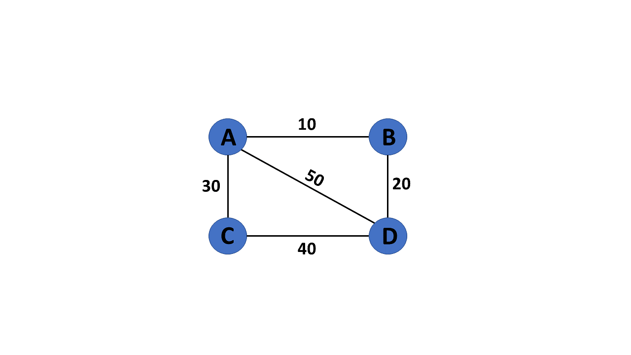
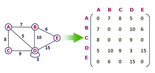
Weighted Graph

In a weighted graph, each edge is assigned a weight or a cost. The weight can be positive, negative or zero. The weight of an edge is represented by a number. A graph G= (V, E) is called a labeled or weighted graph because each edge has a value or weight representing the cost of traversing that edge.

WG = nx.Graph()
WG.add_edges_from([('A', 'B', {"weight": 10}), ('A', 'C', {"weight": 20}), ('B', 'D', {"weight": 30}), ('B', 'E', {"weight": 40}), ('C', 'F', {"weight": 50}), ('C', 'G', {"weight": 60})])
labels = nx.get_edge_attributes(WG, "weight")

Cyclic Graph

A graph is said to be cyclic if it contains a cycle. A cycle is a path of edges that starts and ends on the same vertex. A graph that contains a cycle is called a cyclic graph.

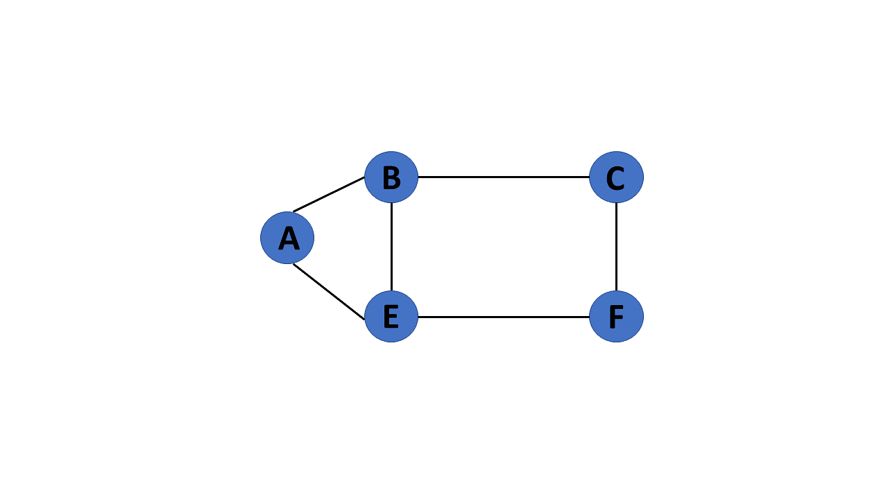
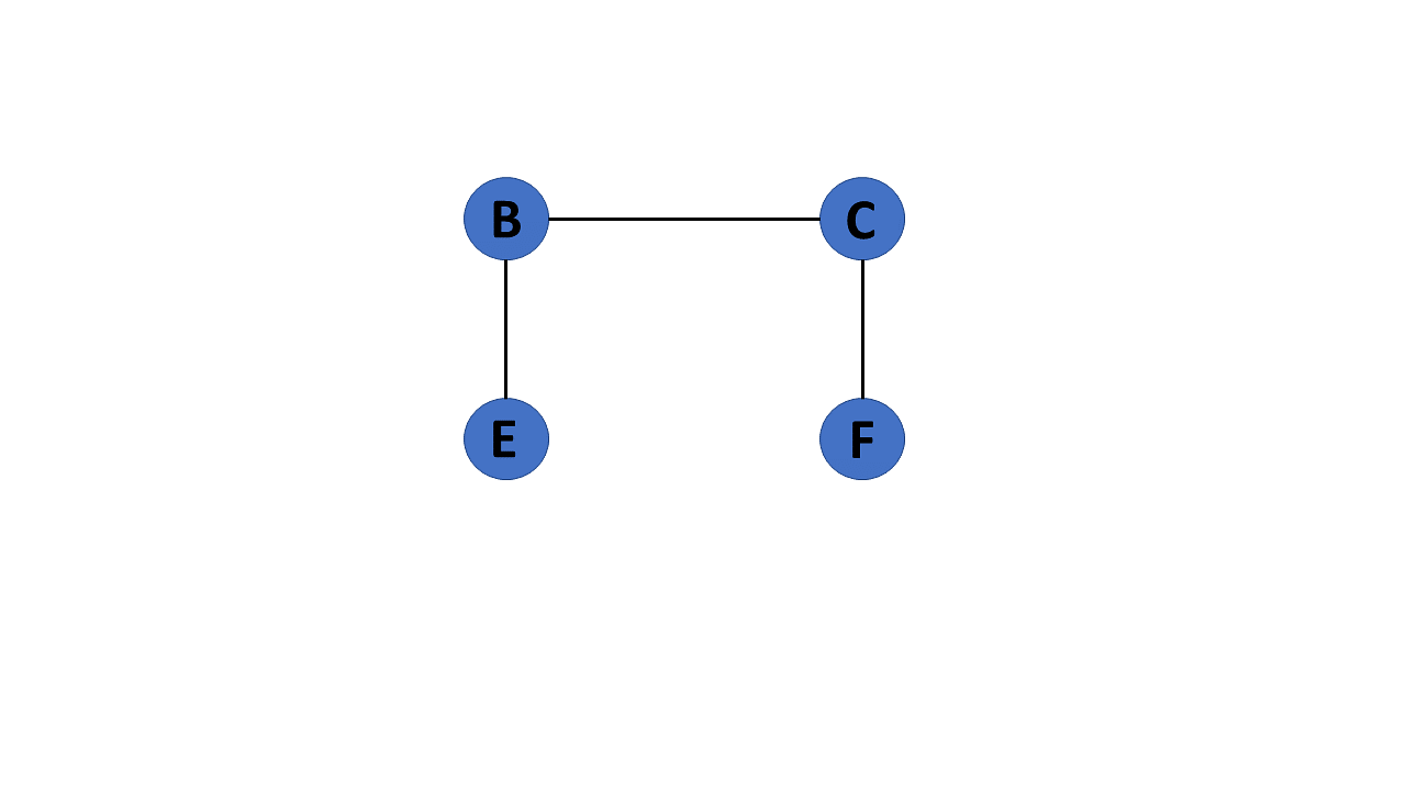
Acyclic Graph

When there are no cycles in a graph, it is called an acyclic graph.

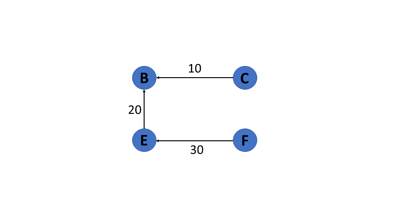
Directed Acyclic Graph

It’s also known as a directed acyclic graph (DAG), and it’s a graph with directed edges but no cycle. It represents the edges using an ordered pair of vertices since it directs the vertices and stores some data.

Trees

A tree is a special type of graph that has a root node, and every node in the graph is connected by edges. It’s a directed acyclic graph with a single root node and no cycles. A tree is a special type of graph that has a root node, and every node in the graph is connected by edges. It’s a directed acyclic graph with a single root node and no cycles.

degree of a vertex

The degree of a vertex is the number of edges incident to it. In the following figure, the degree of vertex A is 3, the degree of vertex B is 4, and the degree of vertex C is 2.

In-Degree and Out-Degree of a Vertex

In a directed graph, the in-degree of a vertex is the number of edges that are incident to the vertex. The out-degree of a vertex is the number of edges that are incident to the vertex.

G = nx.Graph()
G.add_edges_from([('A', 'B'), ('A', 'C'), ('B', 'D'), ('B', 'E'), ('C', 'F'), ('C', 'G')])
print(f"deg(A) = {G.degree['A']}")
DG = nx.DiGraph()
DG.add_edges_from([('A', 'B'), ('A', 'C'), ('B', 'D'), ('B', 'E'), ('C', 'F'), ('C', 'G')])

print(f"deg^-(A) = {DG.in_degree['A']}")
print(f"deg^+(A) = {DG.out_degree['A']}")

Path

A path is a sequence of edges that allows you to go from one vertex to another. The length of a path is the number of edges in it.

Cycle

A cycle is a path that starts and ends at the same vertex.

Graph measures

Degrees and paths can be used to determine the importance of a node in a network. This measure is referred to as centrality

Centrality quantifies the importance of a vertex or node in a network. It helps us to identify key nodes in a graph based on their connectivity and influence on the flow of information or interactions within the network.

Degree centrality

Degree centrality is one of the simplest and most commonly used measures of centrality. It is simply defined as the degree of the node. A high degree centrality indicates that a vertex is highly connected to other vertices in the graph, and thus significantly influences the network.

Closeness centrality

Closeness centrality measures how close a node is to all other nodes in the graph. It corresponds to the average length of the shortest path between the target node and all other nodes in the graph. A node with high closeness centrality can quickly reach all other vertices in the network.

Betweenness centrality

Betweenness centrality measures the number of times a node lies on the shortest path between pairs of other nodes in the graph. A node with high betweenness centrality acts as a bottleneck or bridge between different parts of the graph.

print(f"Degree centrality      = {nx.degree_centrality(G)}")
print(f"Closeness centrality   = {nx.closeness_centrality(G)}")
print(f"Betweenness centrality = {nx.betweenness_centrality(G)}")

The importance of nodes A, B and C in a graph depends on the type of centrality used. Degree centrality considers nodes B and C to be more important because they have more neighbors than node A . However, in closeness centrality, node A is the most important as it can reach any other node in the graph in the shortest possible path. On the other hand, nodes A,B and C have equal betweenness centrality, as they all lie on a large number of shortest paths between other nodes.

Density

The density of a graph is the ratio of the number of edges to the number of possible edges. A graph with high density is considered more connected and has more information flow compared to a graph with low density. A dense graph has a density closer to 1, while a sparse graph has a density closer to 0.

G = nx.Graph()
G.add_edges_from([('A', 'B'), ('A', 'C'), ('B', 'D'), ('B', 'E'), ('C', 'F'), ('C', 'G')])
print(f"Density of G = {nx.density(G)}")

Graph Representation

There are two ways to represent a graph:

Adjacency Matrix
Edge List
Adjacency List

Each data structure has its own advantages and disadvantages that depend on the specific application and requirements.

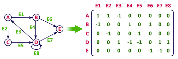
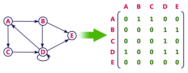
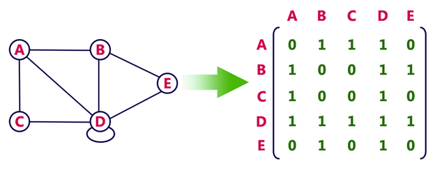
Adjacency Matrix

In an adjacency matrix, each row represents a vertex and each column represents another vertex. If there is an edge between the two vertices, then the corresponding entry in the matrix is 1, otherwise it is 0. The following figure shows an adjacency matrix for a graph with 4 vertices.

drawbacks of adjacency matrix

The adjacency matrix representation of a graph is not suitable for a graph with a large number of vertices. This is because the number of entries in the matrix is proportional to the square of the number of vertices in the graph.
The adjacency matrix representation of a graph is not suitable for a graph with parallel edges. This is because the matrix can only store a single value for each pair of vertices.
One of the main drawbacks of using an adjacency matrix is its space complexity: as the number of nodes in the graph grows, the space required to store the adjacency matrix increases exponentially. adjacency matrix has a space complexity of \(O\left(|V|^2\right)_{\text {, where }}|V|_{\text{repre- }}\) sents the number of nodes in the graph.

Overall, while the adjacency matrix is a useful data structure for representing small graphs, it may not be practical for larger ones due to its space complexity. Additionally, the overhead of adding or removing nodes can make it inefficient for dynamically changing graphs.

Edge list

An edge list is a list of all the edges in a graph. Each edge is represented by a tuple or a pair of vertices. The edge list can also include the weight or cost of each edge. This is the data structure we used to create our graphs with networkx:

edge_list = [(0, 1), (0, 2), (1, 3), (1, 4), (2, 5), (2, 6)]

checking whether two vertices are connected in an edge list requires iterating through the entire list, which can be time-consuming for large graphs with many edges. Therefore, edge lists are more commonly used in applications where space is a concern.

Adjacency List

In an adjacency list, each vertex stores a list of adjacent vertices. The following figure shows an adjacency list for a graph with 4 vertices.

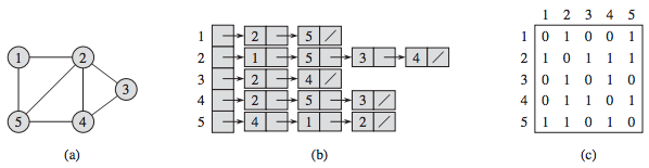
However, checking whether two vertices are connected can be slower than with an adjacency matrix. This is because it requires iterating through the adjacency list of one of the vertices, which can be time-consuming for large graphs.

Graph Traversal

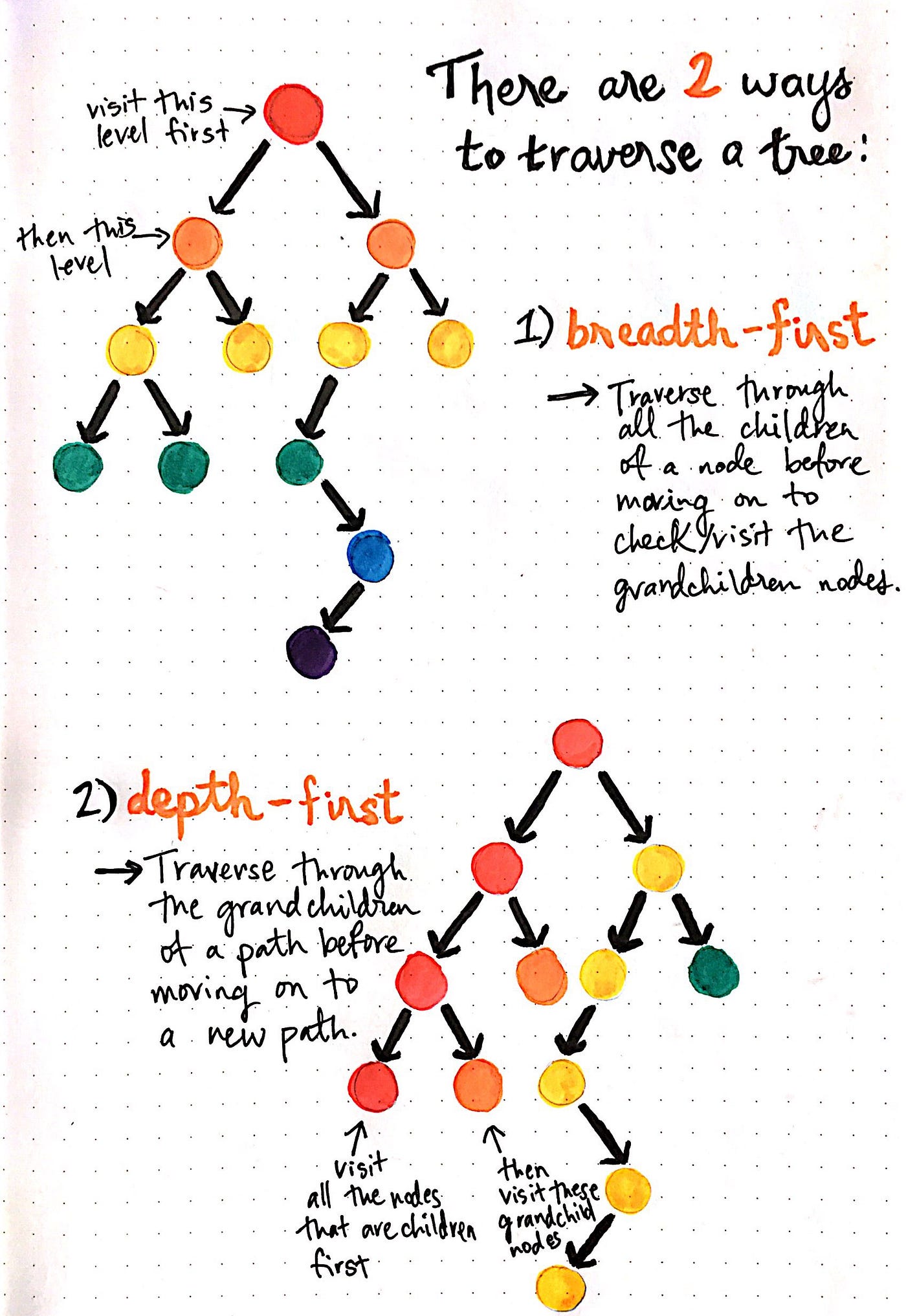
Graph algorithms are critical in solving problems related to graphs, such as finding the shortest path between two nodes or detecting cycles. This section will discuss two graph traversal algorithms: BFS and DFS.

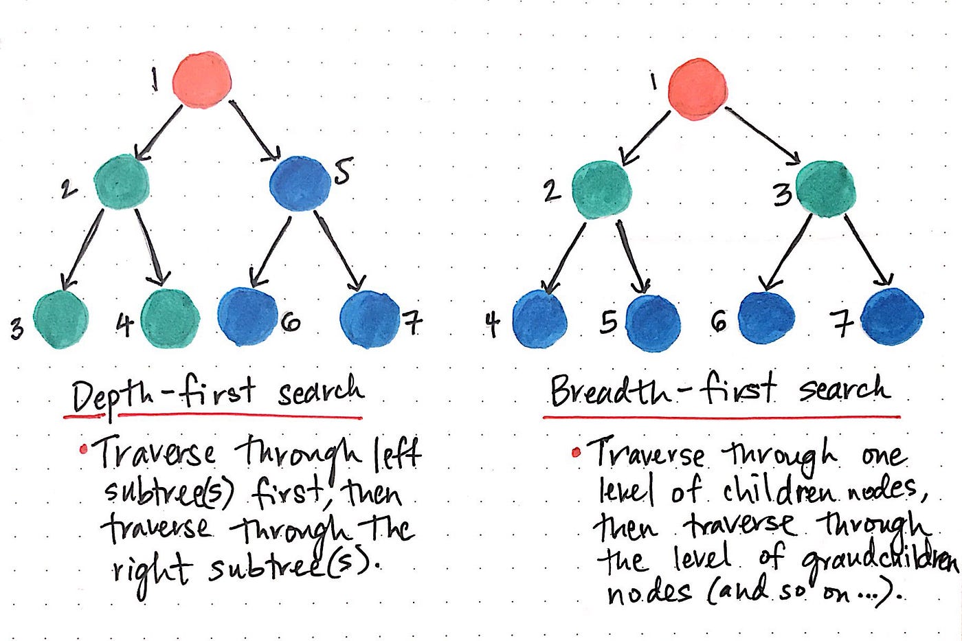
Graph traversal is the process of visiting (checking and/or updating) each vertex in a graph, exactly once. Such traversals are classified by the order in which the vertices are visited. The order may be defined by a specific rule, for example, depth-first search and breadth-first search.

Link: https://medium.com/basecs/breaking-down-breadth-first-search-cebe696709d9

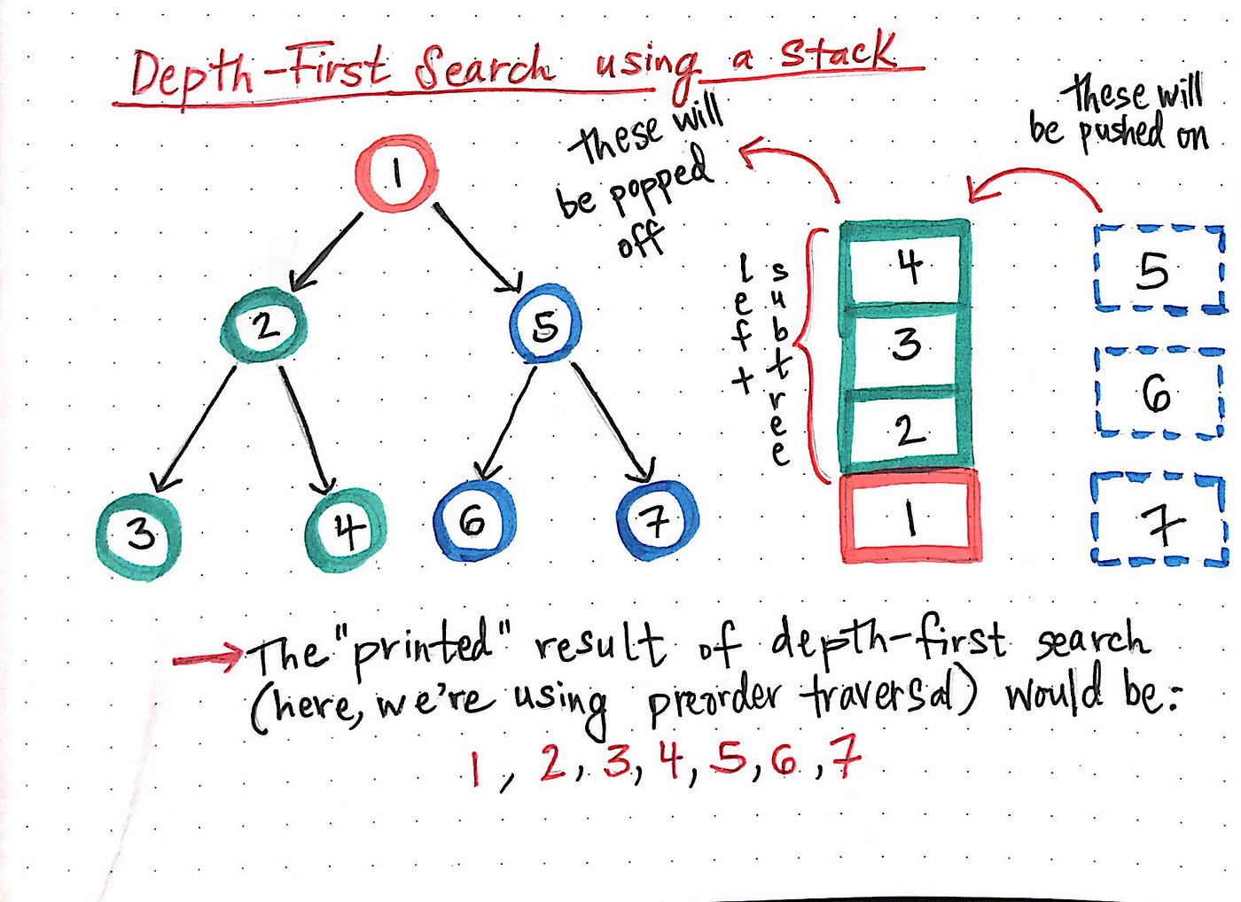
While DFS uses a stack data structure, BFS leans on the queue data structure.

Depth First Search

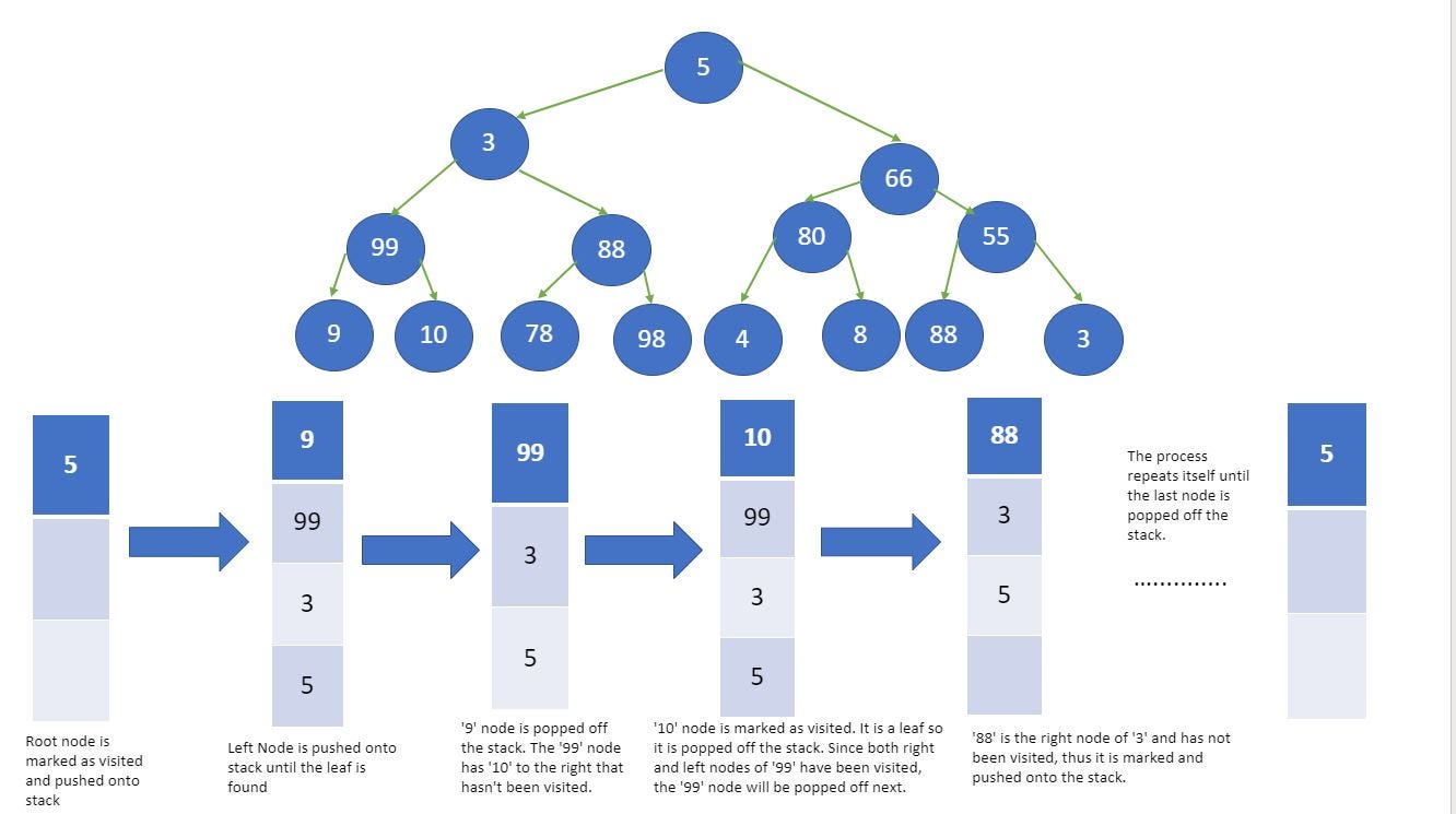
We know that depth-first search is the process of traversing down through one branch of a tree until we get to a leaf, and then working our way back to the “trunk” of the tree. In other words, implementing a DFS means traversing down through the subtrees of a binary search tree.

DFS is a recursive algorithm that starts at the root node and explores as far as possible along each branch before backtracking.

It chooses a node and explores all of its unvisited neighbors, visiting the first neighbor that has not been explored and backtracking only when all the neighbors have been visited. By doing so, it explores the graph by following as deep a path from the starting node as possible before backtracking to explore other branches. This continues until all nodes have been explored.

DFS Algorithm goes ‘deep’ instead of ‘wide’

https://miro.medium.com/v2/resize:fit:1400/1*LUL63FWqneOfsLKqMtHKFw.gif

In depth-first search, once we start down a path, we don’t stop until we get to the end. In other words, we traverse through one branch of a tree until we get to a leaf, and then we work our way back to the trunk of the tree.

Stack data structure is used to implement DFS. The algorithm starts with a particular node of a graph, then goes to any of its adjacent nodes and repeats this process until it finds the goal. If it reaches a node from which there is no unexplored edge leading to an unvisited node, then it backtracks to the last visited node and repeats the process.

G = nx.Graph()
G.add_edges_from([('A', 'B'), ('A', 'C'), ('B', 'D'), ('B', 'E'), ('C', 'F'), ('C', 'G')])

visited = []

def dfs(visited, graph, node):
    if node not in visited:
        visited.append(node)
    # We then iterate through each neighbor of the current node. For each neighbor, we recursively call the dfs() function
    # passing in visited, graph, and the neighbor as arguments:
        for neighbor in graph[node]:
            visited = dfs(visited, graph, neighbor)
    # The dfs() function continues to explore the graph depth-first, visiting all the neighbors of each node until there
    # are no more unvisited neighbors. Finally, the visited list is returned
    return visited

dfs(visited, G, 'A')

Once again, the order we obtained is the one we anticipated in Figure. DFS is useful in solving various problems, such as finding connected components, topological sorting, and solving maze problems. It is particularly useful in finding cycles in a graph since it traverses the graph in a depth-first order, and a cycle exists if, and only if, a node is visited twice during the traversal.

Additionally, many other algorithms in graph theory build upon BFS and DFS, such as Dijkstra’s shortest path algorithm, Kruskal’s minimum spanning tree algorithm, and Tarjan’s strongly connected components algorithm. Therefore, a solid understanding of BFS and DFS is essential for anyone who wants to work with graphs and develop more advanced graph algorithms.

Breadth First Search

Breadth First Search (BFS) is an algorithm for traversing or searching tree or graph data structures. It starts at the tree root (or some arbitrary node of a graph, sometimes referred to as a ‘search key’[1]), and explores the neighbor nodes first, before moving to the next level neighbors.

It works by maintaining a queue of nodes to visit and marking each visited node as it is added to the queue. The algorithm then dequeues the next node in the queue and explores all its neighbors, adding them to the queue if they haven’t been visited yet.

Let’s now see how we can implement it in Python

def bfs(graph, node):
   # We initialize two lists (visited and queue) and add the starting node. The visited list keeps track of the nodes that have been
   # visited #during the search, while the queue list stores the nodes that need to be visited:

   visited, queue = [node], [node]

   while queue:
   # When We enter a while loop that continues until the queue list is empty.
   # Inside the loop, we remove the first node in the queue list using the pop(0) method and store the result in the node variable

       node = queue.pop(0)
       for neighbor in graph[node]:
           if neighbor not in visited:
               visited.append(neighbor)
               queue.append(neighbor)
   # We iterate through the neighbors of the node using a for loop. For each neighbor that has not been visited yet,
   # we add it to the visited list and to the end of the queue list using the append() method. When it’s complete,
   # we return the visited list:
   return visited

bfs(G, 'A')

The order we obtained is the one we anticipated in Figure.

BFS is particularly useful in finding the shortest path between two nodes in an unweighted graph. This is because the algorithm visits nodes in order of their distance from the starting node, so the first time the target node is visited, it must be along the shortest path from the starting node.

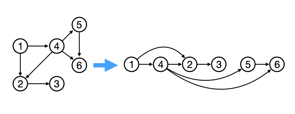
Topological Sort

Topological sorting for Directed Acyclic Graph (DAG) is a linear ordering of vertices such that for every directed edge uv, vertex u comes before v in the ordering. Topological Sorting for a graph is not possible if the graph is not a DAG.

Graph Algorithms

Graph algorithms are used to solve problems that involve graphs. Graph algorithms are used to find the shortest path between two nodes, find the minimum spanning tree, find the strongly connected components, find the shortest path from a single node to all other nodes, find the bridges and articulation points, find the Eulerian path and circuit, find the maximum flow, find the maximum matching, find the biconnected components, find the Hamiltonian path and circuit, find the dominating set, find the shortest path from a single node to all other nodes, find the bridges and articulation points, find the Eulerian path and circuit, find the maximum flow, find the maximum matching, find the biconnected components, find the Hamiltonian path and circuit, find the dominating set, etc.