Continuous Distributions

Definition

A random variable is continuous if possible values comprise either a single interval on the number line or a union of disjoint intervals. X = f(x) is the probability density function of the continues random variable X.

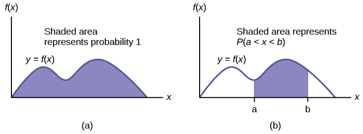
We model a continuous random variable with a curve f(x), called a probability density function (pdf).

Applications

• In the study of the ecology of a lake, a rv X could be the depth measurements at randomly chosen locations.

• In a study of a chemical reaction, Y could be the concentration level of a particular chemical in solution.

• In a study of customer service, W could be the time a customer waits for service.

• f(x) represents the height of the curve at point x.

• For continuous random variables probabilities are areas under the curve.

Attention

We can’t model continuous random variable using discrete rv method.

\[ P(a \leq X \leq b)=\int_{a}^{b} f(x) d x \]

Properties

1. The probability density function \(f:(-\infty, \infty) \rightarrow[0, \infty) \text{ so } f (x) \geq 0\).

2. \(P(-\infty<X<\infty)=\int_{-\infty}^{\infty} f(x) d x=1=P(S)\)

3. \(P(a \leq X \leq b)=\int_{a}^{b} f(x) d x\)

Note

\(P(X=a)=\int_{a}^{a} f(x) d x=0 \text { for all real numbers } a\)

Uniform rv

Random variable \(X \sim U[a,b]\) has the uniform distribution on the interval [a, b] if its density function is

import torch
import matplotlib.pyplot as plt
import seaborn as sns
from scipy.stats import uniform

sns.set_theme(style="darkgrid")

# random numbers from uniform distribution
n = 10000
start = 10
width = 20
data_uniform = uniform.rvs(size=n, loc = start, scale=width)
ax = sns.displot(data_uniform,
                  bins=100,
                  kde=True)
ax.set(xlabel='Uniform Distribution ', ylabel='Frequency')
plt.show()

\[\begin{split} f(x)=\begin{cases} \frac{1}{b - a} & \mathrm{for}\ a \le x \le b, \\[8pt] 0 & \mathrm{for}\ x<a\ \mathrm{or}\ x>b \end{cases} = \frac{1}{b - a} \cdot I_{(a,b)}(x) \end{split}\]

CDF

\[ \begin{align}\begin{aligned} F(x)=P(X \leq x)=\int_{-\infty}^{x} f(t) dt\\= \int_{a}^{x} \frac{1}{b-a} dt \end{aligned}\end{align} \]

\[\begin{split} F(x)= \begin{cases} 0 & \text{for }x < a \\[8pt] \frac{x-a}{b-a} & \text{for }a \le x \le b \\[8pt] 1 & \text{for }x > b \end{cases} \end{split}\]

Expected Value and Variance

\[\begin{split} f(x)=\begin{cases} \frac{1}{b - a} & \mathrm{for}\ a \le x \le b, \\[8pt] 0 & \mathrm{for}\ x<a\ \mathrm{or}\ x>b \end{cases} \end{split}\]

\[\begin{split} \begin{aligned} E(X) &=\int_{a}^{b} x \cdot \frac{1}{b-a} d x=\left.\frac{1}{b-a} \frac{x^{2}}{2}\right|_{a} ^{b}=\frac{b^{2}-a^{2}}{2(b-a)}=\frac{b+a}{2} \\ E\left(X^{2}\right) &=\int_{a}^{b} x^{2} \frac{1}{b-a} d x=\left.\frac{1}{b-a} \frac{x^{3}}{3}\right|_{a} ^{b}=\frac{b^{3}-a^{3}}{3(b-a)}=\frac{b^{2}+a b+a^{2}}{3} \\ V(X) &=E\left(X^{2}\right)-(E(X))^{2} \\ &=\frac{b^{2}+a b+a^{2}}{3}-\left(\frac{b+a}{2}\right)^{2}=\frac{(b-a)^{2}}{12} \end{aligned} \end{split}\]

Example

For random variable \(X \sim U(0,23)\). Find P(2 < X < 18)

\(P(2 < X < 18) = (18-2)\cdot \frac 1 {23-0} = \frac {16}{23}\)

Exponential Distribution

The exponential distribution is a continuous probability distribution that often concerns the amount of time until some specific event happens. It is a process in which events happen continuously and independently at a constant average rate. The exponential distribution has the key property of being memoryless.

Applications

The family of exponential distributions provides probability models that are widely used in engineering and science disciplines to describe time-to-event data.

• Time until birth

• Time until a light bulb fails

• Waiting time in a queue

• Length of service time

• Time between customer arrivals

• the amount of money spent by the customer

• Calculating the time until the radioactive particle decays

PDF

The continuous random variable, say X is said to have an exponential distribution, if it has the following probability density function:

\[\begin{split} \large f(x;\lambda) = \begin{cases} \lambda e^{ - \lambda x} & x \ge 0, \\ 0 & x < 0. \end{cases} =\lambda e^{-\lambda x} I_{(0, \infty)}(x) \end{split}\]

λ is called the distribution rate.

import torch
import matplotlib.pyplot as plt
import seaborn as sns
from scipy.stats import expon

sns.set_theme(style="darkgrid")

data_expon = expon.rvs(scale=1,loc=0,size=1000)
ax = sns.displot(data_expon,
                  kde=True,
                  bins=100)
ax.set(xlabel='Exponential Distribution', ylabel='Frequency')
plt.show()

Expected Value

The mean of the exponential distribution is calculated using the integration by parts.

\[ \begin{align}\begin{aligned}\begin{split} \begin{aligned} &E[X]=\int_{0}^{\infty} x f(x) d x=\int_0^{\infty} x \lambda e^{-\lambda x} d x \\ &=\lambda\left[\left|\frac{-x e^{-\lambda x}}{\lambda}\right|_0^{\infty}+\frac{1}{\lambda} \int_0^{\infty} e^{-\lambda x} d x\right] \\ &=\lambda\left[0+\frac{1}{\lambda} \frac{-e^{-\lambda x}}{\lambda}\right]_0^{\infty} \\ &=\lambda \frac{1}{\lambda^2} \\ &=\frac{1}{\lambda} \end{aligned}\end{split}\\\begin{split}E[X^2]&= \int_{0}^{\infty} x^2 f(x) d x \\ &= \int_{0}^{\infty} x^2 \lambda e^{ - \lambda x} d x \\ &= \frac{2}{\lambda^2} \end{split}\end{aligned}\end{align} \]

Variance

To find the variance of the exponential distribution, we need to find the second moment of the exponential distribution

\[\begin{split} V(X) &= E(X^2) - E(X)^2 \\ &= \frac{2}{\lambda^2} - (\frac{1}{\lambda})^2 \\ &= \frac{1}{\lambda^2} \end{split}\]

Properties

The most important property of the exponential distribution is the memoryless property. This property is also applicable to the geometric distribution.

Normal (Gaussian) Distribution

It is often called Gaussian distribution, in honor of Carl Friedrich Gauss (1777-1855), an eminent German mathematician who gave important contributions towards a better understanding of the normal distribution.

Normal Random Variable

A continuous random variable \(X \sim N(\mu,\sigma^2)\) has the normal distribution with parameters \(\mu\) and \(\sigma^2\) if its density is given by

\[\large f(x)=\frac{1}{\sqrt{2 \pi} \sigma} e^{-(x-\mu)^2 / 2 \sigma^2} \text { for }-\infty<x<\infty\]

A normal distribution is a distribution that is solely dependent on two parameters of the data set: mean and the standard deviation of the sample.

Attention

This characteristic of the distribution makes it extremely simple for statisticians and hence any variable that exhibits normal distribution is feasible to be forecasted with higher accuracy. Essentially, it can help in simplying the model.

Parameters

• Mu is a location parameter. If you change the value of Mu, the entire bell curve is going to slide around.

• If you increase Sigma squared, it’s going to get fatter and therefore shorter because the total area is one, So if it gets fatter, it has to come down. If Sigma squared gets smaller, it’s going to get really tall and thin.

Properties

Normal distribution is simple to explain: Why?

The reasons are:

1. The mean, mode, and median of the distribution are equal.

2. We only need to use the mean and standard deviation to explain the entire distribution.

• f(x) is symmetric around \(x=\mu\) as a consequence, deviations from the mean having the same magnitude.

• f(x) > 0 for all \(x\) and \(\int_{-\infty}^{\infty} f(x) dx = 1\).

• \(\mu + \sigma\) and \(\mu - \sigma\) are inflection points on f(x).

• Mean and median are equal; both are located at the center of the distribution.

Why is it so important

The normal distribution is extremely important because:

• many real-world phenomena involve random quantities that are approximately normal

• it plays a crucial role in the Central Limit Theorem, one of the fundamental results in statistics;

• its great analytical tractability makes it very popular in statistical modelling.

The following variables are close to normally distributed variables:

1. Height of a population

2. Blood pressure of adult human

3. Position of a particle that experiences diffusion

4. Measurement errors

5. Residuals in regression

6. Shoe size of a population

7. Amount of time it takes for employees to reach home

8. A large number of educational measures

But how are so many variables approximately normally distributed?

Let’s consider that the height of a population is a random variable. We can take a sample of heights, plot its distribution and calculate the sample mean. When we repeat this experiment whilst we increase the number of samples then the mean of the samples will end up being very close to normality.

This is known as the Central Limit Theorem.

Probability Density Function

If we plot the normal distribution density function, it’s curve has the following characteristics:

• Mean is the center of the curve. This is the highest point of the curve as most of the points are at the mean.

• There is an equal number of points on each side of the curve. The center of the curve has the most number of points.

• The total area under the curve is the total probability of all of the values that the variable can take.

• The total curve area is therefore 100%

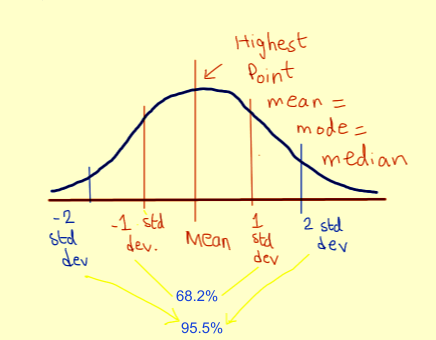
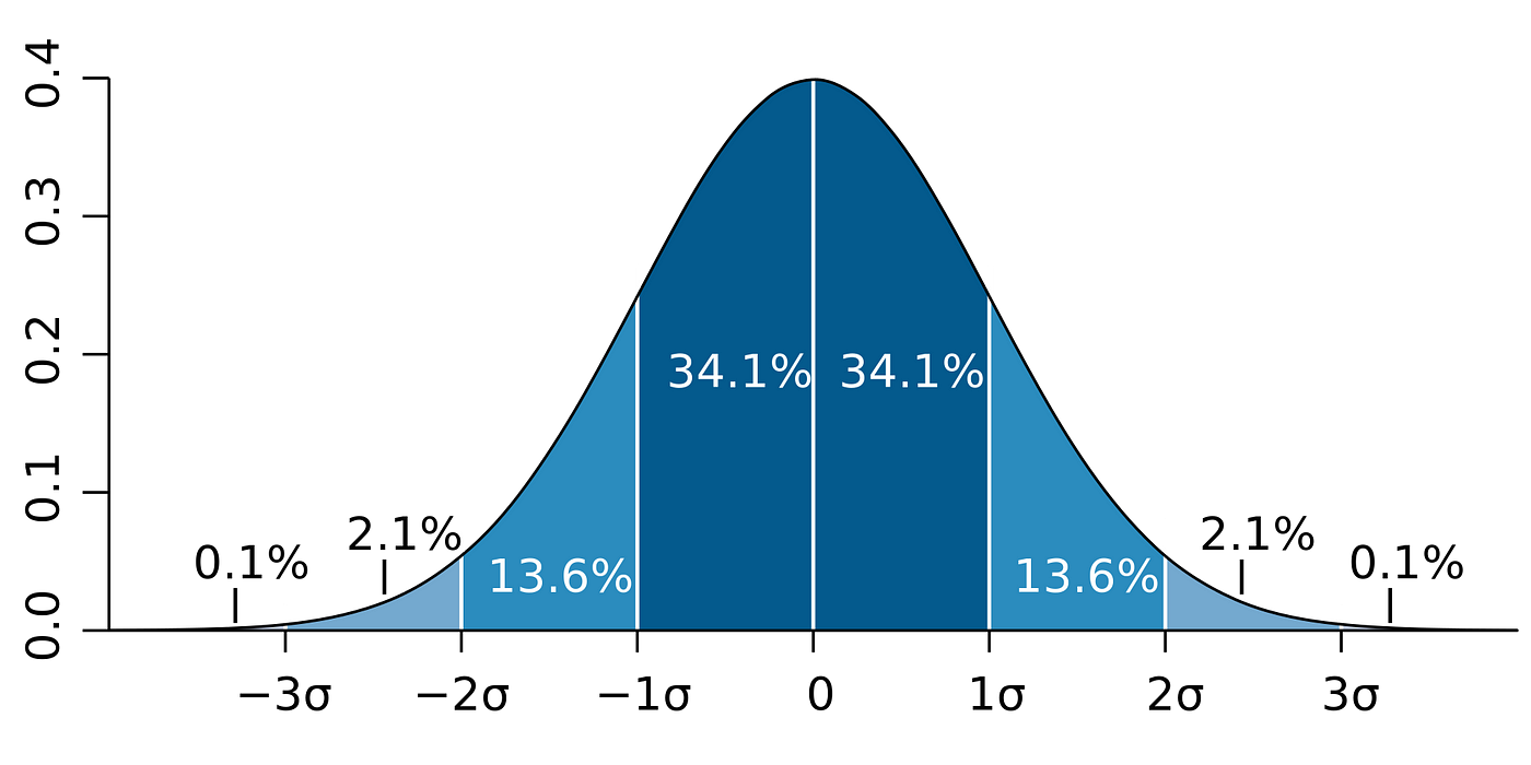
• Approximately 68.2% of all of the points are within the range -1 to 1 standard deviation.

• About 95.5% of all of the points are within the range -2 to 2 standard deviations.

• About 99.7% of all of the points are within the range -3 to 3 standard deviations.

This allows us to easily estimate how volatile a variable is and given a confidence level, what its likely value is going to be. As an instance, in the grey bell-shaped curve above, there is a 68.2% chance that the value of the variable will be within 101–99.

Normal Probability Distribution Function

\[ \large f(x)=\frac{1}{\sqrt{2 \pi} \sigma} e^{-(x-\mu)^{2} / 2 \sigma^{2}} = \frac{1}{\sigma\sqrt{2\pi}} e^{-\frac{1}{2}\left(\frac{x - \mu}{\sigma}\right)^2} \text { for }-\infty<x<\infty \]

import torch
import matplotlib.pyplot as plt
import seaborn as sns
from scipy.stats import norm


sns.set_theme(style="darkgrid")
sample = torch.normal(mean = 8, std = 16, size=(1,1000))

sns.displot(sample[0], kde=True, stat = 'density',)
plt.axvline(torch.mean(sample[0]), color='red', label='mean')

plt.show()

norm.pdf returns a PDF value. The following is the PDF value when 𝑥=1, 𝜇=0, 𝜎=1.

We graph a PDF of the normal distribution using scipy, numpy and matplotlib. We use the domain of −4<𝑥<4, the range of 0<𝑓(𝑥)<0.45, the default values 𝜇=0 and 𝜎=1. plot(x-values,y-values) produces the graph.

print(norm.pdf(x=1.0, loc=0, scale=1))

x = torch.arange(-4,4,0.001)
fig, ax = plt.subplots()

ax.set_title('N(0,$1^2$)')
ax.set_xlabel('x')
ax.set_ylabel('f(x)')
ax.plot(x, norm.pdf(x))
ax.set_ylim(0,0.45)
plt.show()

0.24197072451914337

A normal curve is smooth bell-shaped. It is symmetrical about the 𝑥=𝜇 and has a maximum point at 𝑥=𝜇.

Normal distribution PDF with different standard deviations

Let’s plot the probability distribution functions of a normal distribution where the mean has different standard deviations.

scipy.norm.pdf has keywords, loc and scale. The location (loc) keyword specifies the mean and the scale (scale) keyword specifies the standard deviation.

fig, ax = plt.subplots()
x = torch.arange(-4,4,0.001)

stdvs = [1.0, 2.0, 3.0, 4.0]
for s in stdvs:
    ax.plot(x, norm.pdf(x,scale=s), label='stdv=%.1f' % s)
    
ax.set_xlabel('x')
ax.set_ylabel('pdf(x)')
ax.set_title('Normal Distribution')
ax.legend(loc='best', frameon=True)
ax.set_ylim(0,0.45)
ax.grid(True)

Normal distribution PDF with different means

Let’s plot the probability distribution functions of a normal distribution where the mean has different values.

fig, ax = plt.subplots()
x = torch.linspace(-10,10,100)

means = [0.0, 1.0, 2.0, 5.0]
for mean in means:
    ax.plot(x, norm.pdf(x,loc=mean), label='mean=%.1f' % mean)
    
ax.set_xlabel('x')
ax.set_ylabel('pdf(x)')
ax.set_title('Normal Distribution')
ax.legend(loc='best', frameon=True)
ax.set_ylim(0,0.45)
ax.grid(True)

The mean of the distribution determines the location of the center of the graph. As you can see in the above graph, the shape of the graph does not change by changing the mean, but the graph is translated horizontally.

A cumulative normal distribution function

The cumulative distribution function of a random variable X, evaluated at x, is the probability that X will take a value less than or equal to x. Since the normal distribution is a continuous distribution, the shaded area of the curve represents the probability that X is less or equal than x.

fig, ax = plt.subplots()
# for distribution curve
x= torch.arange(-4,4,0.001)

ax.plot(x, norm.pdf(x))
ax.set_title("Cumulative normal distribution")
ax.set_xlabel('x')
ax.set_ylabel('pdf(x)')
ax.grid(True)
# for fill_between
px=torch.arange(-4,1,0.01)
ax.set_ylim(0,0.5)
ax.fill_between(px,norm.pdf(px),alpha=0.5, color='g')
# for text
ax.text(-1,0.1,"cdf(x)", fontsize=20)
plt.show()

Expected Value and Variance

\(E(X) = \mu\)

\(V(X) = \sigma^2\)

Problems With Normality

Assuming normality has its own flaws. As an instance, we cannot assume that the stock price follows normal distribution as the price cannot be negative. Therefore the stock price potentially follows a log of the normal distribution to ensure it is never below zero.

We know that the daily returns can be negative, therefore the returns can at times follow a normal distribution. It is not wise to assume that the variable follows a normal distribution without any analysis.

A variable can follow Poisson, Student-t, or Binomial distribution as an instance and falsely assuming that a variable follows normal distribution can lead to inaccurate results.

Identify the Normal RV?

Many methods exist for testing whether a variable has a normal distribution

1. Histogram

The histogram is a data visualization that shows the distribution of a variable. It is a bar graph that shows the frequency of each value in the variable. The histogram is a graphical representation of the distribution of a variable.

sample = torch.normal(mean = 8, std = 16, size=(1,1000))
sample2 = torch.distributions.uniform.Uniform(2,3).sample([1,1000])

sns.displot(sample[0], kde=True,).set(title='Normal Distribution')
plt.axvline(torch.mean(sample[0]), color='red', label='mean')

sns.displot(sample2[0], kde=True,).set(title='Uniform Distribution')
plt.show()

2. Box Plot

The Box Plot is another visualization technique that can be used for detecting non-normal samples.

The box plot is a graphical representation of the distribution of a variable. It is a graphical representation of the five-number summary of a variable. The five-number summary is the minimum, first quartile, median, third quartile, and maximum of a variable.

3. QQ Plot

QQ Plot stands for Quantile vs Quantile Plot, which is exactly what it does: plotting theoretical quantiles against the actual quantiles of our variable.

The QQ Plot allows us to see deviation of a normal distribution much better than in a Histogram or Box Plot.

Standard Normal Distribution

The normal distribution with parameter values \(\mu\) = 0 and \(\sigma^2\) = 1 is called the standard normal distribution.

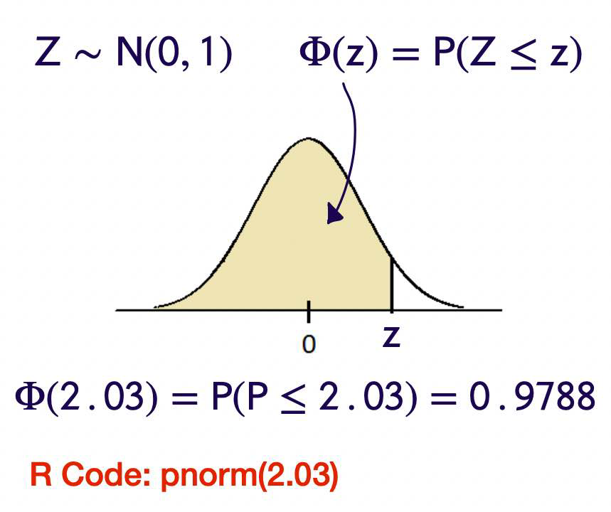
A rv with the standard normal distribution is denoted by \(Z \sim N(0, 1)\)

If \(X \sim N\left(\mu, \sigma^2\right)\) then

\[ f_X(x)=\frac{1}{\sqrt{2 \pi} \sigma} e^{-(x-\mu)^2 / 2 \sigma^2} \text { for }-\infty<x<\infty \]

If \(Z \sim N(0,1)\) then

\[ f_Z(x)=\frac{1}{\sqrt{2 \pi}} e^{-x^2 / 2} \text { for }-\infty<x<\infty \]

PDF

\(f_{Z}(x)=\frac{1}{\sqrt{2 \pi}} e^{-x^{2} / 2} \text { for }-\infty<x<\infty\)

Cumulative distribution function

We use special notation to denote the cdf of the standard normal curve

\(F(z)=\Phi(z)=P(Z \leq z)=\int_{-\infty}^{z} \frac{1}{\sqrt{2 \pi}} e^{-x^{2} / 2} d x\)

Properties

1. The standard normal density function is symmetric about the y axis.

2. The standard normal distribution rarely occurs naturally.

3. Instead, it is a reference distribution from which information about other normal distributions can be obtained via a simple formula.

4. The cdf of the standard normal, \(\Phi(z)\) can be found in tables and it can also be computed with a single command in R.

5. As we’ll see, sums of standard normal random variables play a large role in statistical analysis.

Proposition

\(\text { If } X \sim N\left(\mu, \sigma^{2}\right), \text { then } \frac{X-\mu}{\sigma} \sim N(0,1)\)

\(\frac{X-\mu}{\sigma}\) Shifted by \(\mu\) or (Centered at zero) and scaled by \(\frac{1}{\sigma}\) that will give us variance of 1.

\(\mathrm{Z} \sim \mathrm{N}(0,1) \Rightarrow \sigma \mathrm{Z}+\mu \sim \mathrm{N}\left(\mu, \sigma^2\right)\)

Example

Let \(X \sim N(2,3)\)

\[\begin{split} \begin{aligned} P ( X \leq 4.1) &= P \left(\frac{ X -\mu}{\sigma} \leq \frac{4.1-2}{\sqrt{3}}\right) \\ &= P ( Z \leq 1.21) \end{aligned} \end{split}\]

Proving this proposition

For any continuous random variable. Suppose we have Y rv, with Desnity function \(f_{Y}(y)\)

We know

\(P(y \leqslant a)=\int_{-\infty}^{a} f_{y}(y) d y\)

What if

\(P(2y \leqslant a)\)

= Can’t really use the density function until we isolate y =

\(P\left(y \leq \frac{a}{2}\right) = \int_{-\infty}^{a / 2} f_{y}(y) d y\)

This true for all transformation of Y.

With \(P\left(\frac{x-\mu}{\sigma} \leq a\right)=P(x \leq a \sigma+\mu) = \int_{x}^{a \sigma+\mu} \frac{1}{\sqrt{2 \pi} \sigma} e^{-(x-\mu)^{2} / 2 \sigma^{2}}\)

U subsitution

Let

\(u=\frac{x-\mu}{\sigma}\)

\(d u=\frac{1}{\sigma} d x\)

SO \(= \int_{-\infty}^{a} \frac{1}{\sqrt{2 \pi}} e^{-u^{2} / 2} d u\) This is density function for N(0,1).

Examples

Find P(X<2) when N(3, 2)?

In norm.cdf, the location (loc) keyword specifies the mean and the scale (scale) keyword specifies the standard deviation.

from scipy.stats import norm

val = norm.cdf(x=2, loc=3, scale=2)

print(f"P(X<2) = {val}")


fig, ax = plt.subplots()

x= torch.arange(-4,10,0.001)
ax.plot(x, norm.pdf(x,loc=3,scale=2))
ax.set_title("N(3,$2^2$)")
ax.set_xlabel('x')
ax.set_ylabel('pdf(x)')
ax.grid(True)
# for fill_between
px=torch.arange(-4,2,0.01)
ax.set_ylim(0,0.25)
ax.fill_between(px,norm.pdf(px,loc=3,scale=2),alpha=0.5, color='g')
# for text
ax.text(-0.5,0.02,round(val,2), fontsize=20)
plt.show()

P(X<2) = 0.3085375387259869

\[\begin{split} \begin{aligned} \mathrm{P}(\mathrm{X} \leq 2) &=\mathrm{P}\left(\frac{\mathrm{X}-\mu}{\sigma} \leq \frac{2-3}{\sqrt{2}}\right) \\ &=\mathrm{P}(\mathrm{Z} \leq 1.21) \\ & \approx 0.30 \end{aligned} \end{split}\]

R code: pnorm(1.2)

Find P(X<4.1) when N(2, 3)?

Let \(X \sim N(2,3)\). Then

\[\begin{split} \begin{aligned} P ( X \leq 4.1) &= P \left(\frac{ X -\mu}{\sigma} \leq \frac{4.1-2}{\sqrt{3}}\right) \\ &= P (Z \leq 1.21) \\ & \approx 0.8868 \end{aligned} \end{split}\]

R Code: pnorm(1.21)

z_score <- (4.1 - 2) / sqrt(3)
pnorm(z_score)

\[\begin{split} \begin{aligned} & X _1, X _2, \ldots, X _{10} \stackrel{ id }{\sim} N (2,3) \\ &\overline{ X } \sim N \left(\mu, \sigma^2 / n \right)= N (2,3 / 10) \\ & P (\overline{ X } \leq 2.3)= P \left(\frac{\overline{ X }-\mu_{\overline{ X }}}{\sigma_{\overline{ X }}} \leq \frac{2.3-2}{\sqrt{3 / 10}}\right) \\ &\frac{\overline{ X -\mu}}{\sigma / \sqrt{ n }}=\begin{aligned} &= P ( Z \leq 0.5477) \\ & \approx 0.7081 \end{aligned} \end{aligned} \end{split}\]

Interval between variables

To find the probability of an interval between certain variables, you need to subtract cdf from another cdf.

Let’s find 𝑃(0.5<𝑋<2) with a mean of 1 and a standard deviation of 2.

print(norm(1, 2).cdf(2) - norm(1,2).cdf(0.5))

0.2901687869569368

\[ X \sim N\left(1,2^2\right), P(0.5<X<2) \]

fig, ax = plt.subplots()

# for distribution curve
x= torch.arange(-6,8,0.001)
ax.plot(x, norm.pdf(x,loc=1,scale=2))
ax.set_title("N(1,$2^2$)")
ax.set_xlabel('x')
ax.set_ylabel('pdf(x)')
ax.grid(True)
px=torch.arange(0.5,2,0.01)
ax.set_ylim(0,0.25)
ax.fill_between(px,norm.pdf(px,loc=1,scale=2),alpha=0.5, color='g')
pro=norm(1, 2).cdf(2) - norm(1,2).cdf(0.5)
ax.text(0.2,0.02,round(pro,2), fontsize=20)
plt.show()

P(Z > 1.25) ?

Let’s plot a graph.

fig, ax = plt.subplots()
x= torch.arange(-4,4,0.01)
gr4sf=norm.sf(x=1.25, loc=0, scale=1)
print(gr4sf)

ax.plot(x, norm.pdf(x,loc=0,scale=1))
ax.set_title("N(0,$1^2$)")

ax.set_xlabel('x')
ax.set_ylabel('pdf(x)')

ax.grid(True)
px=torch.arange(1.25,4,0.01)
#ax.set_ylim(0,0.15)
ax.fill_between(px,norm.pdf(px,loc=0,scale=1),alpha=0.5, color='g')
ax.text(1.25,0.02,"sf(x) %.2f" %(gr4sf), fontsize=20)
plt.show()

0.10564977366685535

we can use sf which is called the survival function and it returns 1-cdf.

If X = N(1, 4), find P(0 < X < 3.2)?

\[\begin{split} P(0 \leq X \leq 3.2)&=\int_{0}^{3.2} f_{X}(x) d x \\ &=P\left(\frac{0-1}{2} \leqslant \frac{x-1}{2} \leqslant \frac{3.2-1}{2}\right) \\ &=P\left(-\frac{1}{2} \leq Z \leq 1.1\right)\\ &=P(z \leq 1.1)-P\left(z<-\frac{1}{2}\right)\\ &=\Phi(1.1)-\Phi\left(-\frac{1}{2}\right)\\ &= .558 \end{split}\]

print(norm(1, 2).cdf(3.2) - norm(1,2).cdf(0))

0.5557964003276304

fig, ax = plt.subplots()

# for distribution curve
x= torch.arange(-6,8,0.001)
ax.plot(x, norm.pdf(x,loc=1,scale=2))
ax.set_title("N(1,$2^2$)")
ax.set_xlabel('x')
ax.set_ylabel('pdf(x)')
ax.grid(True)
px=torch.arange(0.5,2,0.01)
ax.set_ylim(0,0.25)
ax.fill_between(px,norm.pdf(px,loc=1,scale=2),alpha=0.5, color='g')
pro=norm(1, 2).cdf(3.5) - norm(1,2).cdf(0)
ax.text(0.2,0.02,round(pro,2), fontsize=20)
plt.show()

Gamma Distribution

The gamma distribution term is mostly used as a distribution which is defined as two parameters – shape parameter and inverse scale parameter, having continuous probability distributions. Its importance is largely due to its relation to exponential and normal distributions.

Gamma distributions have two free parameters, named as alpha (α) and beta (β), where;

• α = Shape parameter

• β = Rate parameter (the reciprocal of the scale parameter)

The scale parameter β is used only to scale the distribution. This can be understood by remarking that wherever the random variable x appears in the probability density, then it is divided by β. Since the scale parameter provides the dimensional data, it is seldom useful to work with the “standard” gamma distribution, i.e., with β = 1.

Gamma function:

The gamma function \([10]\), shown by \(\Gamma( x )\), is an extension of the factorial function to real (and complex) numbers. Specifically, if \(n \in\{1,2,3, \ldots\}\), then

\[ \Gamma( n )=( n -1) ! \]

Probability Density Function

\[ f(x)=\frac{1}{\Gamma(\alpha)} \beta^\alpha x^{\alpha-1} e^{-\beta x } \]

Mean

\[\begin{split} \begin{aligned} \mu &= E [ X ]=\int_{-\infty}^{\infty} xf ( x ) dx \\ &=\int_0^{\infty} x \frac{1}{\Gamma(\alpha)} \beta^\alpha x ^{\alpha-1} e ^{-\beta x } dx \\ &=\frac{\alpha}{\beta} \end{aligned} \end{split}\]

Variance

\[\begin{split} \begin{aligned} \sigma^2=\operatorname{Var}[ X ] &= E \left[( X -\mu)^2\right] \\ &= E \left[ X ^2\right]-( E [ X ])^2 \\ &=\cdots=\frac{\alpha}{\beta^2} \end{aligned} \end{split}\]

Chi-squared Distribution

One Parameter:

• degrees of freedom: \(n \geq 1\) ( \(n\) is an integer) \(X \sim \chi^2(n)\) is defined as \(\Gamma\left(\frac{n}{2}, \frac{1}{2}\right)\)

mean

\[ \mu= E [ X ]= n \]

variance

\[ \sigma^2=\operatorname{Var}[ X ]=2 n \]

T-distribution

Let \(Z \sim N(0,1)\) and \(W \sim \chi^2(n)\) be independent random variables. Define

\[ T =\frac{ Z }{\sqrt{ W / n }} \]

the t-distribution Write \(X \sim t ( n )\) One Parameter: degrees of freedom: \(n \geq 1\) ( \(n\) is an integer) The pdf:

\[\begin{split} \begin{array}{r} f(x)=\frac{\Gamma\left(\frac{n+1}{2}\right)}{\sqrt{\pi n} \Gamma\left(\frac{n}{2}\right)}\left(1+\frac{x^2}{n}\right)^{-(n+1) / 2} \\ -\infty<x<\infty \end{array} \end{split}\]