Logistic Regression

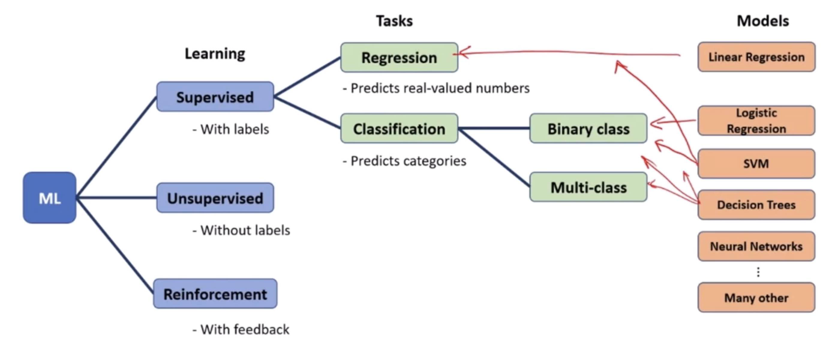
Logistic regression is a statistical method for analyzing a dataset in which there are one or more independent variables that determine an outcome. The outcome is measured with a dichotomous variable (in which there are only two possible outcomes). It’s used extensively for binary classification problems, such as spam detection (spam or not spam), loan default (default or not), disease diagnosis (positive or negative), etc. Logistic regression predicts the probability that a given input belongs to a certain category.

Sigmoid / Logistic Function :

The core of logistic regression is the sigmoid function, which maps any real-valued number into a value between 0 and 1, making it suitable for probability estimation. The sigmoid function is defined as \(\sigma(z) = \frac{1}{1 + e^{-z}}\), where \(z\) is the input to the function, often \(z = w^T x + b\), with \(w\) being the weights, \(x\) the input features, and \(b\) the bias.

Cost / loss Function:

MLE in Binary Classification

Maximum Likelihood Estimation (MLE) is a central concept in statistical modeling, including binary classification tasks. Binary classification involves predicting whether an instance belongs to one of two classes (e.g., spam or not spam, diseased or healthy) based on certain input features.

In binary classification, you often model the probability of the positive class (\(y=1\)) as a function of input features (\(X\)) using a logistic function, leading to logistic regression. The probability that a given instance belongs to the positive class can be expressed as:

\[ P(Y=1 | X; \theta) = \frac{1}{1 + e^{-(\beta_0 + \beta_1X_1 + ... + \beta_nX_n)}} \]

Here, \(\theta\) represents the model parameters (\(\beta_0, \beta_1, ..., \beta_n\)), and \(X_1, ..., X_n\) are the input features.

The likelihood function \(L(\theta)\) in the context of binary classification is the product of the probabilities of each observed label, given the input features and the model parameters. For a dataset with \(m\) instances, where \(y_i\) is the label of the \(i\)-th instance, and \(p_i\) is the predicted probability of the \(i\)-th instance being in the positive class, the likelihood is:

\[ L(\theta) = \prod_{i=1}^{m} p_i^{y_i} (1-p_i)^{1-y_i} \]

This product is maximized when the model parameters (\(\theta\)) are such that the predicted probabilities (\(p_i\)) are close to 1 for actual positive instances and close to 0 for actual negative instances.

Log-Likelihood:

To simplify calculations and handle numerical stability, we use the log-likelihood, which converts the product into a sum:

\[ \ell(\theta) = \sum_{i=1}^{m} \left[ y_i \log(p_i) + (1-y_i) \log(1-p_i) \right] \]

The goal is to find the parameters (\(\theta\)) that maximize this log-likelihood.

Threshold Decision:

The probability outcome from the sigmoid function is converted into a binary outcome via a threshold decision rule, usually 0.5 (if the sigmoid output is greater than or equal to 0.5, the outcome is classified as 1, otherwise as 0).

Performance Metrics:

Here are some performance metrics that can be used to evaluate the performance of a binary classifier:

Accuracy
Precision
Recall
F1 score
ROC curve
Confusion matrix
AUC (Area Under the Curve)

Logistic Regression in PyTorch:

Here’s a simple example of how to implement logistic regression in PyTorch. PyTorch is a deep learning framework that provides a lot of flexibility and capabilities, including automatic differentiation which is handy for logistic regression.

Step 1: Import Libraries

import torch
import torch.nn as nn
import torch.optim as optim

Step 2: Create Dataset

For simplicity, let’s assume a binary classification task with some synthetic data.

# Features [sample size, number of features]
X = torch.tensor([[1, 2], [4, 5], [7, 8], [9, 10]], dtype=torch.float32)
# Labels [sample size, 1]
y = torch.tensor([[0], [1], [1], [0]], dtype=torch.float32)

Step 3: Define the Model

class LogisticRegressionModel(nn.Module):
    def __init__(self, input_size, num_classes):
        super(LogisticRegressionModel, self).__init__()
        self.linear = nn.Linear(input_size, num_classes)
    
    def forward(self, x):
        out = torch.sigmoid(self.linear(x))
        return out

Step 4: Instantiate Model, Loss, and Optimizer

input_size = 2
num_classes = 1
model = LogisticRegressionModel(input_size, num_classes)

criterion = nn.BCELoss()
optimizer = optim.SGD(model.parameters(), lr=0.01)

Step 5: Train the Model

num_epochs = 100
for epoch in range(num_epochs):
    # Forward pass
    outputs = model(X)
    loss = criterion(outputs, y)
    
    # Backward and optimize
    optimizer.zero_grad()
    loss.backward()
    optimizer.step()
    
    if (epoch+1) % 10 == 0:
        print(f'Epoch [{epoch+1}/{num_epochs}], Loss: {loss.item():.4f}')

This code snippet demonstrates the essential parts of implementing logistic regression in PyTorch, including model definition, data preparation, loss computation, and the training loop. After training, the model’s weights are adjusted to minimize the loss, making the model capable of predicting the probability that a new, unseen input belongs to a certain category.