Graph
A graph is a non-linear data structure consisting of nodes and edges. The nodes are sometimes also referred to as vertices and the edges are lines or arcs that connect any two nodes in the graph. More formally a Graph can be defined as, a Graph consists of a finite set of vertices(or nodes) and set of Edges which connect a pair of nodes.
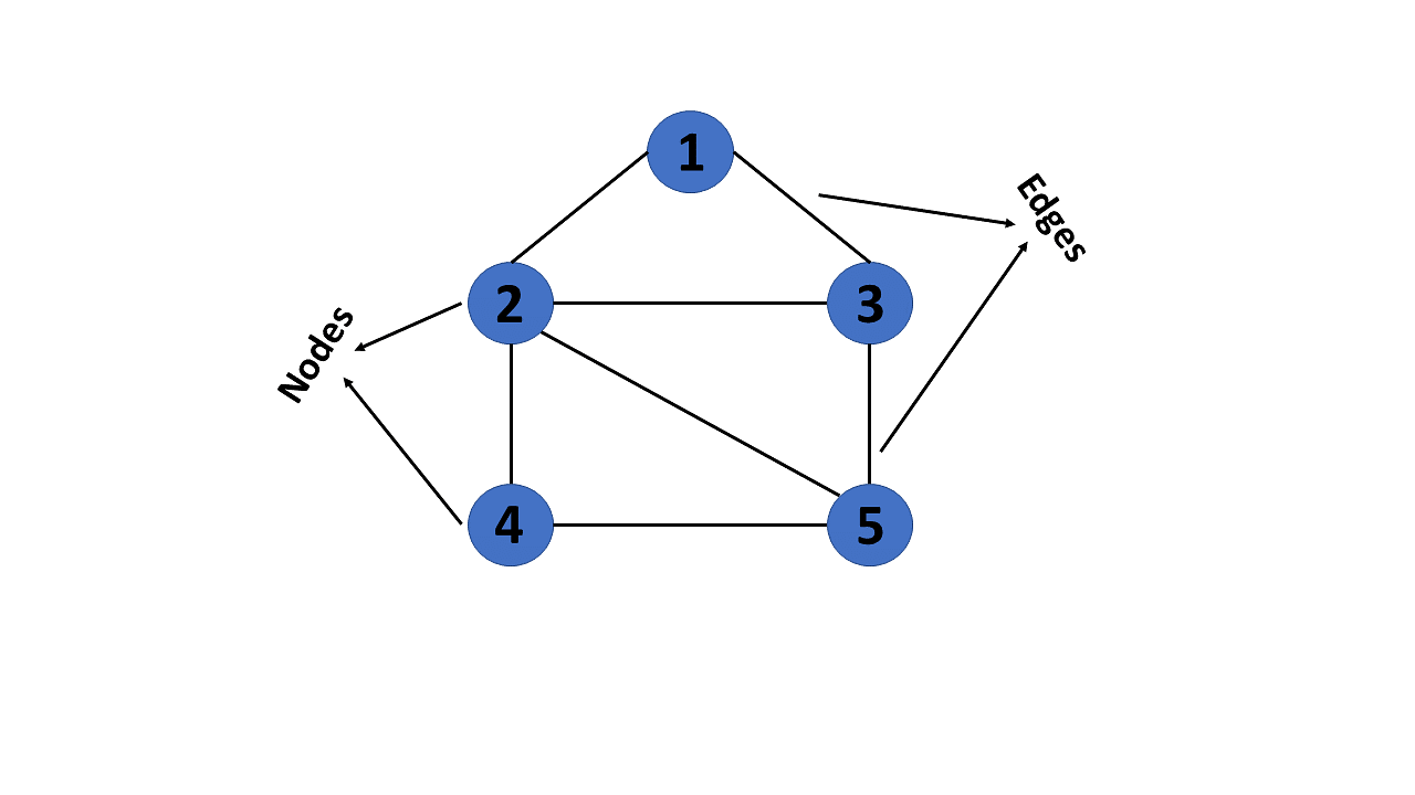
In graph theory, a graph is a mathematical structure consisting of a set of objects, called vertices or nodes, and a set of connections, called edges, which link pairs of vertices. The notation:
is used to represent a graph, where \(G\) is the graph, \(V\) is the set of vertices, and \(\bigvee\) is the set of edges.
The nodes of a graph can represent any objects, such as cities, people, web pages, or molecules, and the edges represent the relationships or connections between them.
import networkx as nx
import matplotlib.pyplot as plt

G = nx.Graph()
G.add_edges_from([('A', 'B'), ('A', 'C'), ('B', 'D'), ('B', 'E'), ('C', 'F'), ('C', 'G')])

plt.axis('off')
nx.draw_networkx(G,
                 pos=nx.spring_layout(G, seed=0),
                 node_size=600,
                 cmap='coolwarm',
                 font_size=14,
                 font_color='white'
                 )
/home/docs/checkouts/readthedocs.org/user_builds/ml-math/envs/latest/lib/python3.11/site-packages/networkx/drawing/nx_pylab.py:1497: UserWarning: No data for colormapping provided via 'c'. Parameters 'cmap' will be ignored
  node_collection = ax.scatter(

Terminology
The following are the most commonly used terms in graph theory with respect to graphs:
Vertex - A vertex, also called a “node”, is a fundamental part of a graph. In the context of graphs, a vertex is an object which may contain zero or more items called attributes.
Edge - An edge is a connection between two vertices. An edge may contain a weight/value/cost.
Path - A path is a sequence of edges connecting a sequence of vertices.
Cycle - A cycle is a path of edges that starts and ends on the same vertex.
Weighted Graph/Network - A weighted graph is a graph with numbers assigned to its edges. These numbers are called weights.
Unweighted Graph/Network - An unweighted graph is a graph in which all edges have equal weight.
Directed Graph/Network - A directed graph is a graph where all the edges are directed.
Undirected Graph/Network - An undirected graph is a graph where all the edges are not directed.
Adjacent Vertices - Two vertices in a graph are said to be adjacent if there is an edge connecting them.
Types of Graphs
There are two types of graphs:
Directed Graphs
Undirected Graphs
Weighted Graph
Cyclic Graph
Acyclic Graph
Directed Acyclic Graph
Directed Graphs
In a directed graph, all the edges are directed. That means, each edge is associated with a direction. For example, if there is an edge from node A to node B, then the edge is directed from A to B and not the other way around.
Directed graph, also called a digraph.
DG = nx.DiGraph()
DG.add_edges_from([('A', 'B'), ('A', 'C'), ('B', 'D'),
('B', 'E'), ('C', 'F'), ('C', 'G')])
nx.draw_networkx(DG, pos=nx.spring_layout(DG, seed=0), node_size=600, cmap='coolwarm', font_size=14, font_color='white')

Undirected Graphs
In an undirected graph, all the edges are undirected. That means, each edge is associated with a direction. For example, if there is an edge from node A to node B, then the edge is directed from A to B and not the other way around.
G = nx.Graph()
G.add_edges_from([('A', 'B'), ('A', 'C'), ('B', 'D'),
('B', 'E'), ('C', 'F'), ('C', 'G')])

nx.draw_networkx(G, pos=nx.spring_layout(G, seed=0), node_size=600, cmap='coolwarm', font_size=14, font_color='white')

Weighted Graph
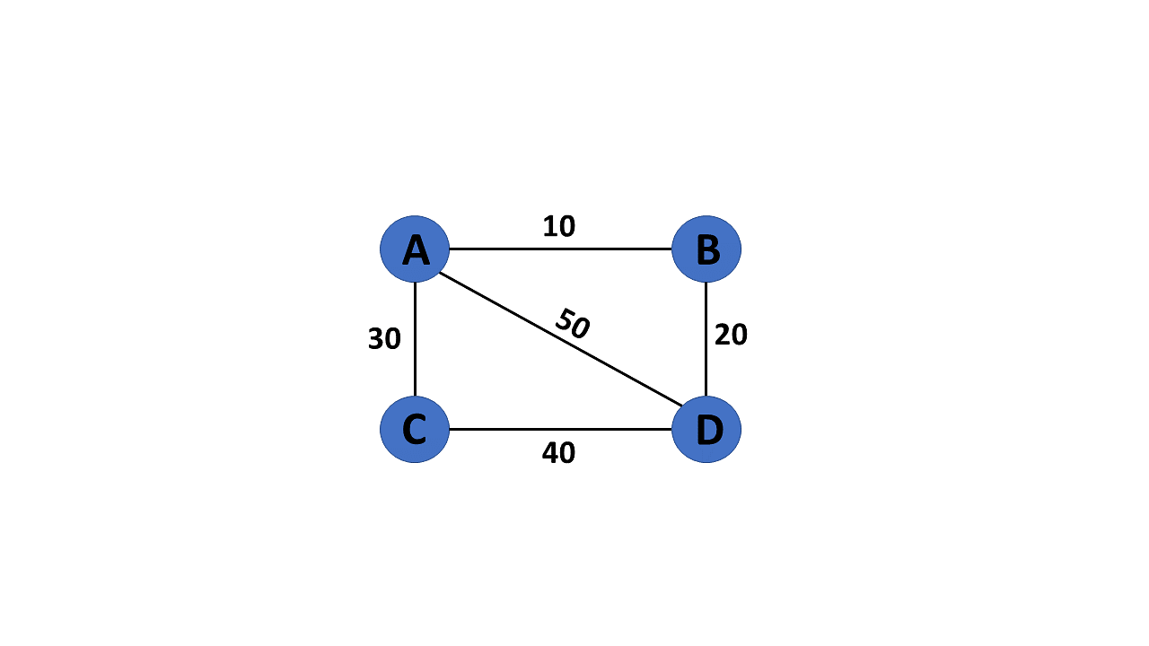
In a weighted graph, each edge is assigned a weight or a cost. The weight can be positive, negative or zero. The weight of an edge is represented by a number. A graph G= (V, E) is called a labeled or weighted graph because each edge has a value or weight representing the cost of traversing that edge.
WG = nx.Graph()
WG.add_edges_from([('A', 'B', {"weight": 10}), ('A', 'C', {"weight": 20}), ('B', 'D', {"weight": 30}), ('B', 'E', {"weight": 40}), ('C', 'F', {"weight": 50}), ('C', 'G', {"weight": 60})])
labels = nx.get_edge_attributes(WG, "weight")
Cyclic Graph
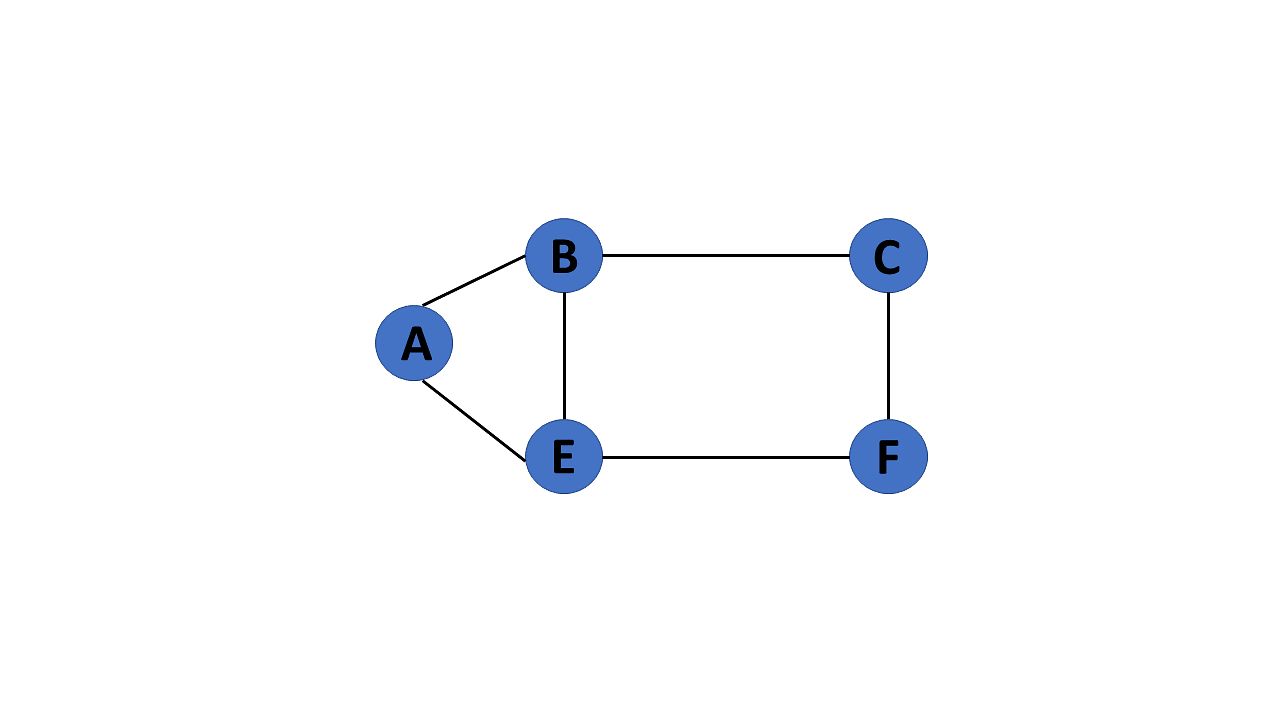
A graph is said to be cyclic if it contains a cycle. A cycle is a path of edges that starts and ends on the same vertex. A graph that contains a cycle is called a cyclic graph.
Acyclic Graph
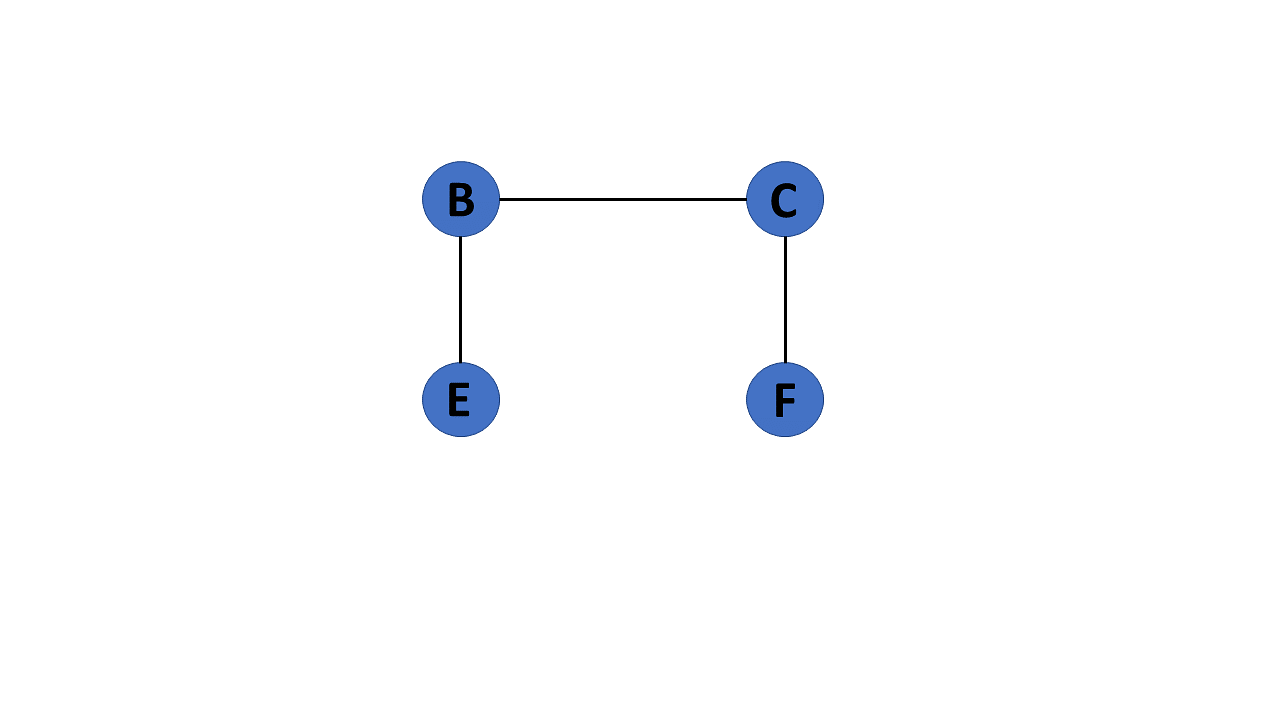
When there are no cycles in a graph, it is called an acyclic graph.
Directed Acyclic Graph
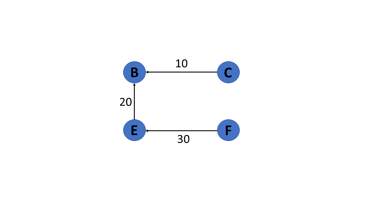
It’s also known as a directed acyclic graph (DAG), and it’s a graph with directed edges but no cycle. It represents the edges using an ordered pair of vertices since it directs the vertices and stores some data.
Trees
A tree is a special type of graph that has a root node, and every node in the graph is connected by edges. It’s a directed acyclic graph with a single root node and no cycles. A tree is a special type of graph that has a root node, and every node in the graph is connected by edges. It’s a directed acyclic graph with a single root node and no cycles.
degree of a vertex
The degree of a vertex is the number of edges incident to it. In the following figure, the degree of vertex A is 3, the degree of vertex B is 4, and the degree of vertex C is 2.
In-Degree and Out-Degree of a Vertex
In a directed graph, the in-degree of a vertex is the number of edges that are incident to the vertex. The out-degree of a vertex is the number of edges that are incident to the vertex.

G = nx.Graph()
G.add_edges_from([('A', 'B'), ('A', 'C'), ('B', 'D'), ('B', 'E'), ('C', 'F'), ('C', 'G')])
print(f"deg(A) = {G.degree['A']}")
DG = nx.DiGraph()
DG.add_edges_from([('A', 'B'), ('A', 'C'), ('B', 'D'), ('B', 'E'), ('C', 'F'), ('C', 'G')])

print(f"deg^-(A) = {DG.in_degree['A']}")
print(f"deg^+(A) = {DG.out_degree['A']}")
deg(A) = 2
deg^-(A) = 0
deg^+(A) = 2
Path
A path is a sequence of edges that allows you to go from one vertex to another. The length of a path is the number of edges in it.
Cycle
A cycle is a path that starts and ends at the same vertex.
Graph measures
Degrees and paths can be used to determine the importance of a node in a network. This measure is referred to as centrality
Centrality quantifies the importance of a vertex or node in a network. It helps us to identify key nodes in a graph based on their connectivity and influence on the flow of information or interactions within the network.
Degree centrality
Degree centrality is one of the simplest and most commonly used measures of centrality. It is simply defined as the degree of the node. A high degree centrality indicates that a vertex is highly connected to other vertices in the graph, and thus significantly influences the network.
Closeness centrality
Closeness centrality measures how close a node is to all other nodes in the graph. It corresponds to the average length of the shortest path between the target node and all other nodes in the graph. A node with high closeness centrality can quickly reach all other vertices in the network.
Betweenness centrality
Betweenness centrality measures the number of times a node lies on the shortest path between pairs of other nodes in the graph. A node with high betweenness centrality acts as a bottleneck or bridge between different parts of the graph.
The importance of nodes A, B and C in a graph depends on the type of centrality used. Degree centrality considers nodes B and C to be more important because they have more neighbors than node A . However, in closeness centrality, node A is the most important as it can reach any other node in the graph in the shortest possible path. On the other hand, nodes A,B and C have equal betweenness centrality, as they all lie on a large number of shortest paths between other nodes.
Density
The density of a graph is the ratio of the number of edges to the number of possible edges. A graph with high density is considered more connected and has more information flow compared to a graph with low density. A dense graph has a density closer to 1, while a sparse graph has a density closer to 0.
print(f"Degree centrality      = {nx.degree_centrality(G)}")
print(f"Closeness centrality   = {nx.closeness_centrality(G)}")
print(f"Betweenness centrality = {nx.betweenness_centrality(G)}")

G = nx.Graph()
G.add_edges_from([('A', 'B'), ('A', 'C'), ('B', 'D'), ('B', 'E'), ('C', 'F'), ('C', 'G')])
print(f"Density of G = {nx.density(G)}")
Degree centrality      = {'A': 0.3333333333333333, 'B': 0.5, 'C': 0.5, 'D': 0.16666666666666666, 'E': 0.16666666666666666, 'F': 0.16666666666666666, 'G': 0.16666666666666666}
Closeness centrality   = {'A': 0.6, 'B': 0.5454545454545454, 'C': 0.5454545454545454, 'D': 0.375, 'E': 0.375, 'F': 0.375, 'G': 0.375}
Betweenness centrality = {'A': 0.6, 'B': 0.6, 'C': 0.6, 'D': 0.0, 'E': 0.0, 'F': 0.0, 'G': 0.0}
Density of G = 0.2857142857142857
Graph Representation
There are two ways to represent a graph:
Adjacency Matrix
Edge List
Adjacency List
Each data structure has its own advantages and disadvantages that depend on the specific application and requirements.
Adjacency Matrix
In an adjacency matrix, each row represents a vertex and each column represents another vertex. If there is an edge between the two vertices, then the corresponding entry in the matrix is 1, otherwise it is 0. The following figure shows an adjacency matrix for a graph with 4 vertices.
drawbacks of adjacency matrix
The adjacency matrix representation of a graph is not suitable for a graph with a large number of vertices. This is because the number of entries in the matrix is proportional to the square of the number of vertices in the graph.
The adjacency matrix representation of a graph is not suitable for a graph with parallel edges. This is because the matrix can only store a single value for each pair of vertices.
One of the main drawbacks of using an adjacency matrix is its space complexity: as the number of nodes in the graph grows, the space required to store the adjacency matrix increases exponentially. adjacency matrix has a space complexity of \(O\left(|V|^2\right)_{\text {, where }}|V|_{\text{repre- }}\) sents the number of nodes in the graph.
Overall, while the adjacency matrix is a useful data structure for representing small graphs, it may not be practical for larger ones due to its space complexity. Additionally, the overhead of adding or removing nodes can make it inefficient for dynamically changing graphs.
Edge list
An edge list is a list of all the edges in a graph. Each edge is represented by a tuple or a pair of vertices. The edge list can also include the weight or cost of each edge. This is the data structure we used to create our graphs with networkx:
edge_list = [(0, 1), (0, 2), (1, 3), (1, 4), (2, 5), (2, 6)]
checking whether two vertices are connected in an edge list requires iterating through the entire list, which can be time-consuming for large graphs with many edges. Therefore, edge lists are more commonly used in applications where space is a concern.
Adjacency List
In an adjacency list, each vertex stores a list of adjacent vertices. The following figure shows an adjacency list for a graph with 4 vertices.
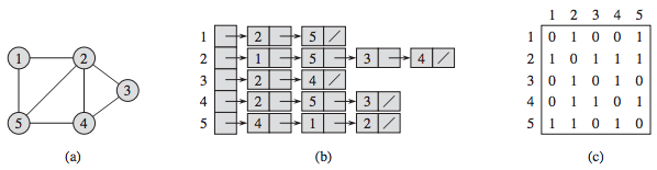
However, checking whether two vertices are connected can be slower than with an adjacency matrix. This is because it requires iterating through the adjacency list of one of the vertices, which can be time-consuming for large graphs.
Graph Traversal
Graph algorithms are critical in solving problems related to graphs, such as finding the shortest path between two nodes or detecting cycles. This section will discuss two graph traversal algorithms: BFS and DFS.
Graph traversal is the process of visiting (checking and/or updating) each vertex in a graph, exactly once. Such traversals are classified by the order in which the vertices are visited. The order may be defined by a specific rule, for example, depth-first search and breadth-first search.
Link: https://medium.com/basecs/breaking-down-breadth-first-search-cebe696709d9
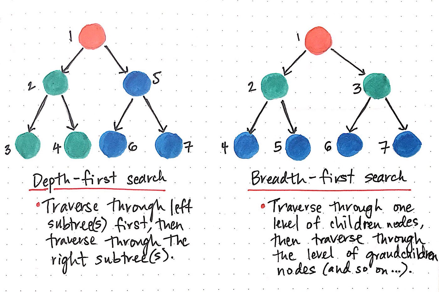
While DFS uses a stack data structure, BFS leans on the queue data structure.
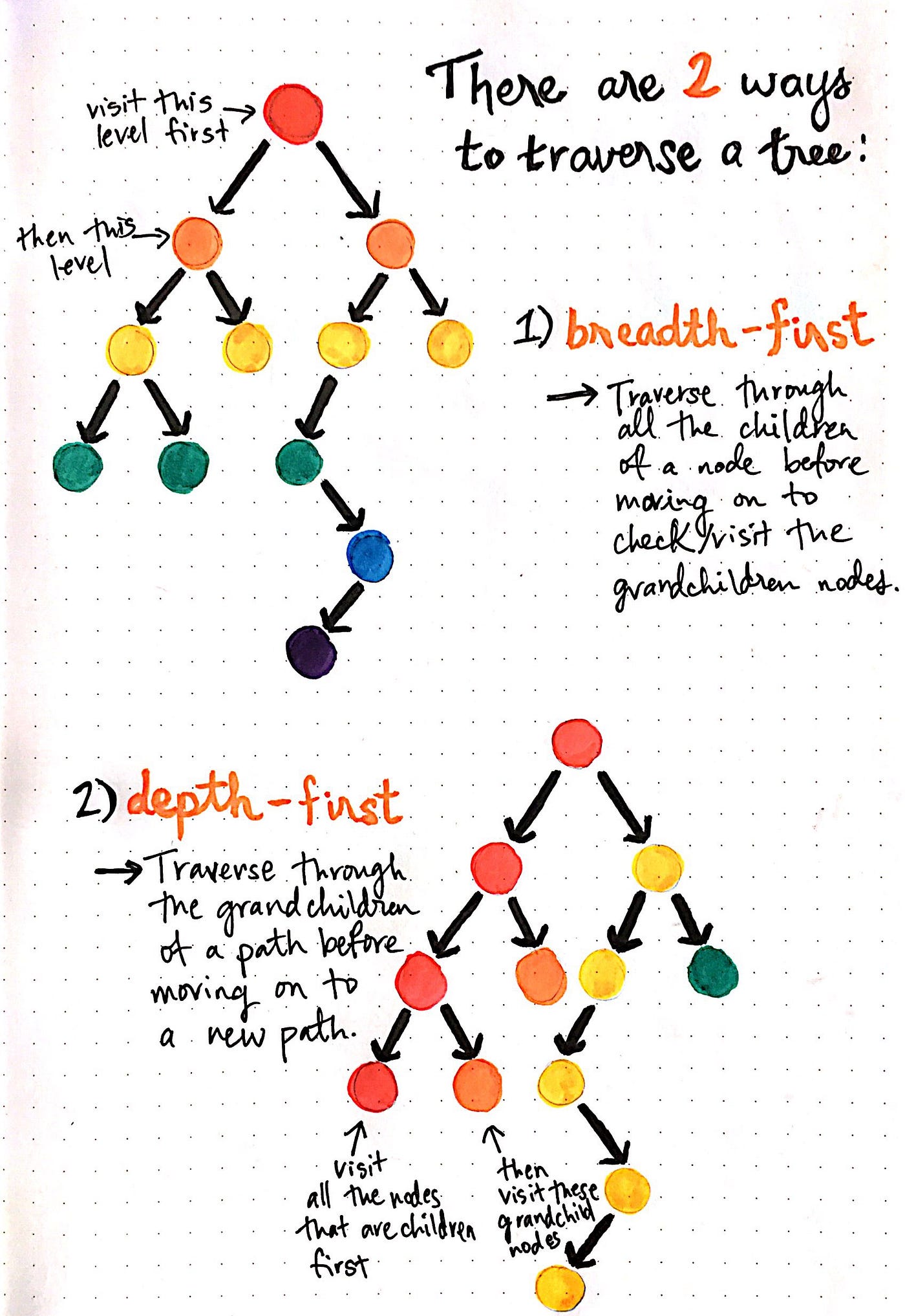
Depth First Search
We know that depth-first search is the process of traversing down through one branch of a tree until we get to a leaf, and then working our way back to the “trunk” of the tree. In other words, implementing a DFS means traversing down through the subtrees of a binary search tree.
DFS is a recursive algorithm that starts at the root node and explores as far as possible along each branch before backtracking.
It chooses a node and explores all of its unvisited neighbors, visiting the first neighbor that has not been explored and backtracking only when all the neighbors have been visited. By doing so, it explores the graph by following as deep a path from the starting node as possible before backtracking to explore other branches. This continues until all nodes have been explored.
DFS Algorithm goes ‘deep’ instead of ‘wide’
https://miro.medium.com/v2/resize:fit:1400/1*LUL63FWqneOfsLKqMtHKFw.gif
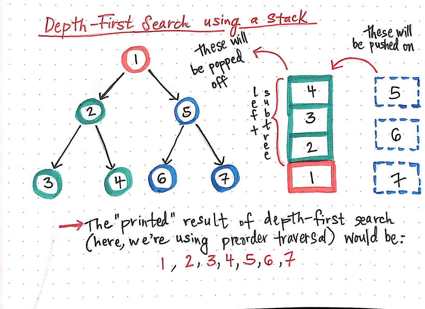
In depth-first search, once we start down a path, we don’t stop until we get to the end. In other words, we traverse through one branch of a tree until we get to a leaf, and then we work our way back to the trunk of the tree.
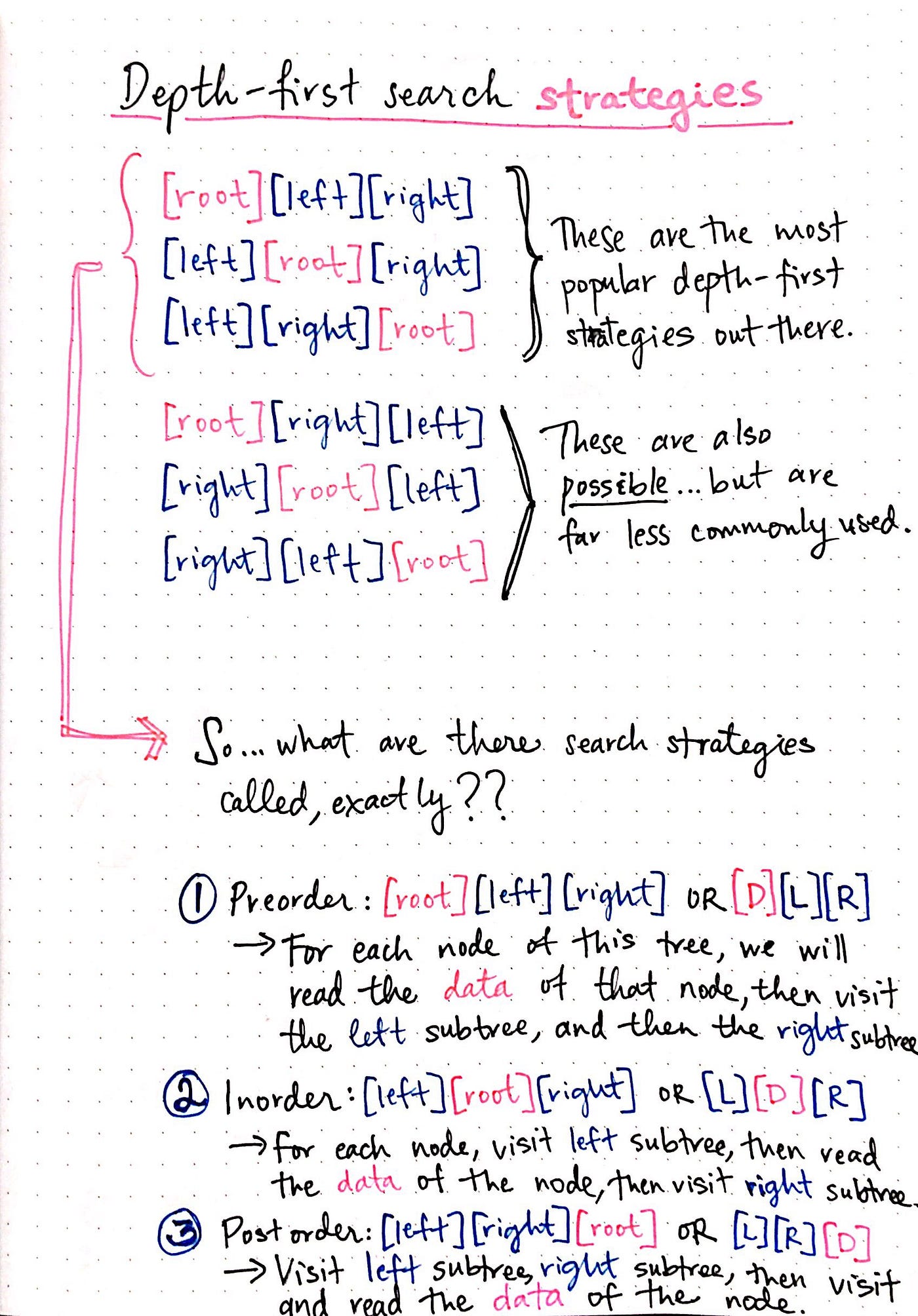
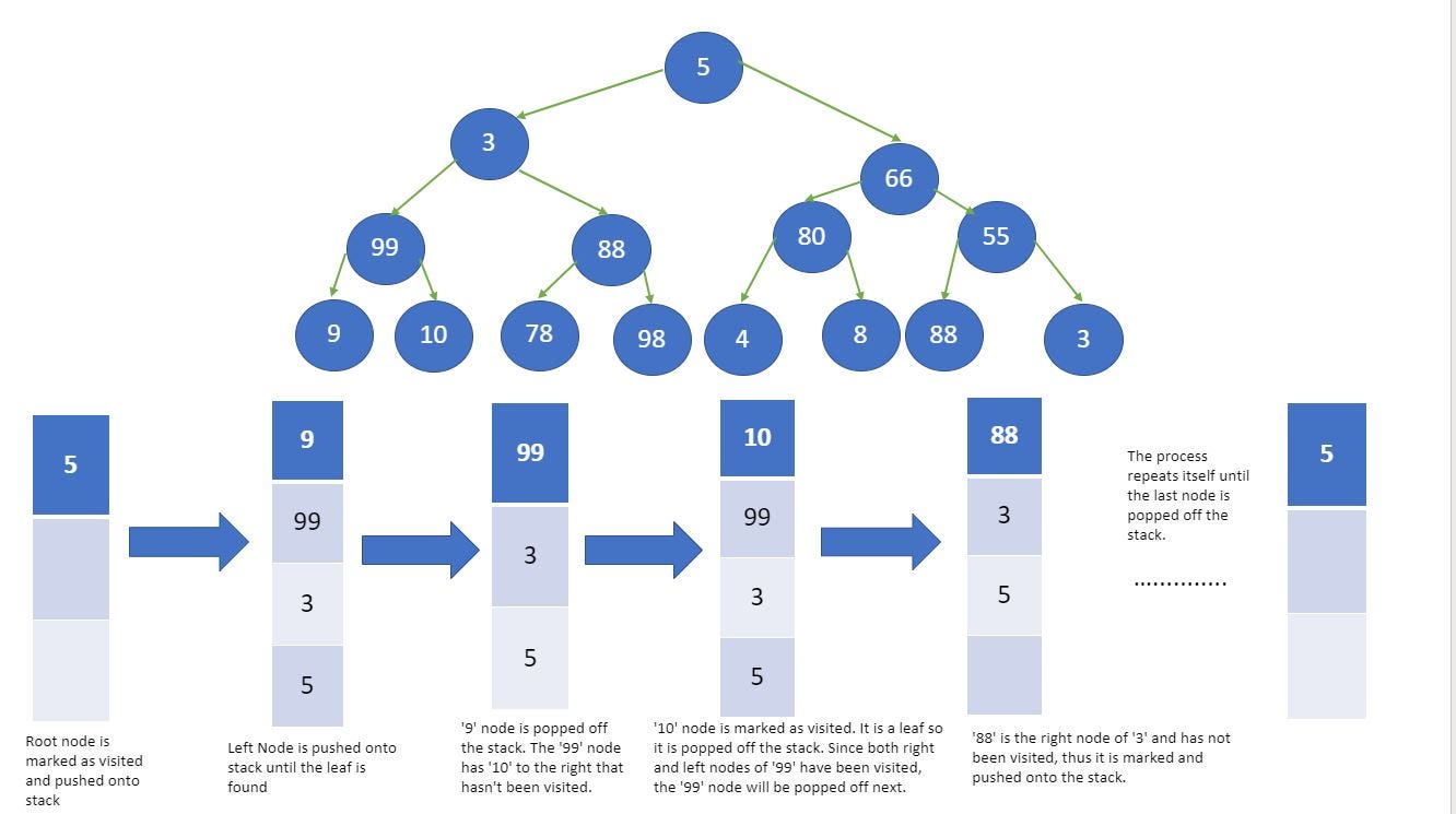
Stack data structure is used to implement DFS. The algorithm starts with a particular node of a graph, then goes to any of its adjacent nodes and repeats this process until it finds the goal. If it reaches a node from which there is no unexplored edge leading to an unvisited node, then it backtracks to the last visited node and repeats the process.
G = nx.Graph()
G.add_edges_from([('A', 'B'), ('A', 'C'), ('B', 'D'), ('B', 'E'), ('C', 'F'), ('C', 'G')])

visited = []

def dfs(visited, graph, node):
    if node not in visited:
        visited.append(node)
    # We then iterate through each neighbor of the current node. For each neighbor, we recursively call the dfs() function
    # passing in visited, graph, and the neighbor as arguments:
        for neighbor in graph[node]:
            visited = dfs(visited, graph, neighbor)
    # The dfs() function continues to explore the graph depth-first, visiting all the neighbors of each node until there
    # are no more unvisited neighbors. Finally, the visited list is returned
    return visited

dfs(visited, G, 'A')
['A', 'B', 'D', 'E', 'C', 'F', 'G']

Once again, the order we obtained is the one we anticipated in Figure. DFS is useful in solving various problems, such as finding connected components, topological sorting, and solving maze problems. It is particularly useful in finding cycles in a graph since it traverses the graph in a depth-first order, and a cycle exists if, and only if, a node is visited twice during the traversal.
Additionally, many other algorithms in graph theory build upon BFS and DFS, such as Dijkstra’s shortest path algorithm, Kruskal’s minimum spanning tree algorithm, and Tarjan’s strongly connected components algorithm. Therefore, a solid understanding of BFS and DFS is essential for anyone who wants to work with graphs and develop more advanced graph algorithms.
Breadth First Search
Breadth First Search (BFS) is an algorithm for traversing or searching tree or graph data structures. It starts at the tree root (or some arbitrary node of a graph, sometimes referred to as a ‘search key’[1]), and explores the neighbor nodes first, before moving to the next level neighbors.
It works by maintaining a queue of nodes to visit and marking each visited node as it is added to the queue. The algorithm then dequeues the next node in the queue and explores all its neighbors, adding them to the queue if they haven’t been visited yet.
Let’s now see how we can implement it in Python
def bfs(graph, node):
    # We initialize two lists (visited and queue) and add the starting node. The visited list keeps track of the nodes that have been
    # visited #during the search, while the queue list stores the nodes that need to be visited:

    visited, queue = [node], [node]

    while queue:
    # When We enter a while loop that continues until the queue list is empty.
    # Inside the loop, we remove the first node in the queue list using the pop(0) method and store the result in the node variable

        node = queue.pop(0)
        for neighbor in graph[node]:
            if neighbor not in visited:
                visited.append(neighbor)
                queue.append(neighbor)
    # We iterate through the neighbors of the node using a for loop. For each neighbor that has not been visited yet,
    # we add it to the visited list and to the end of the queue list using the append() method. When it’s complete,
    # we return the visited list:
    return visited

bfs(G, 'A')
['A', 'B', 'C', 'D', 'E', 'F', 'G']

The order we obtained is the one we anticipated in Figure.
BFS is particularly useful in finding the shortest path between two nodes in an unweighted graph. This is because the algorithm visits nodes in order of their distance from the starting node, so the first time the target node is visited, it must be along the shortest path from the starting node.
Topological Sort
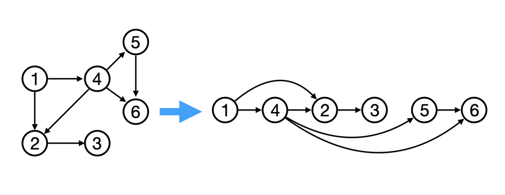
Topological sorting for Directed Acyclic Graph (DAG) is a linear ordering of vertices such that for every directed edge uv, vertex u comes before v in the ordering. Topological Sorting for a graph is not possible if the graph is not a DAG.
Graph Algorithms
Graph algorithms are used to solve problems that involve graphs. Graph algorithms are used to find the shortest path between two nodes, find the minimum spanning tree, find the strongly connected components, find the shortest path from a single node to all other nodes, find the bridges and articulation points, find the Eulerian path and circuit, find the maximum flow, find the maximum matching, find the biconnected components, find the Hamiltonian path and circuit, find the dominating set, find the shortest path from a single node to all other nodes, find the bridges and articulation points, find the Eulerian path and circuit, find the maximum flow, find the maximum matching, find the biconnected components, find the Hamiltonian path and circuit, find the dominating set, etc.
Recursion
Recursion is a fundamental programming concept where a function calls itself to solve smaller instances of the same problem until a base condition is met. It’s a powerful tool for tackling problems that can be broken down into similar sub-problems, such as traversing data structures like trees and graphs.
Recursion involves a function calling itself directly or indirectly to solve a problem. Each recursive call works on a smaller portion of the problem, moving towards a base case that stops the recursion.
Key Components of Recursion:
Base Case: The condition under which the recursion stops.
Recursive Case: The part of the function where it calls itself with a modified parameter.
How Recursion Works: The Call Stack
When a recursive function is invoked, each call is placed on the call stack until it reaches the base case. After hitting the base case, the stack unwinds as each call returns its result.
def factorial(n):
    if n == 0 or n == 1:  # Base case
        return 1
    else:
        return n * factorial(n - 1)  # Recursive call
Call Stack for
factorial(3):factorial(3)waits forfactorial(2)factorial(2)waits forfactorial(1)factorial(1)returns1(base case)
factorial(2)computes2 * 1 = 2and returns2
factorial(3)computes3 * 2 = 6and returns6
Recursion Depth and Stack Limitations
Python imposes a recursion depth limit (default is around 1000) to prevent infinite recursions from causing a stack overflow.
Checking Recursion Limit:
import sys
print(sys.getrecursionlimit())
Setting a New Recursion Limit:
sys.setrecursionlimit(2000)
Warning: Increasing the recursion limit can lead to a crash if the system runs out of memory.
When to Use Recursion
Divide and Conquer Algorithms: Such as quicksort and mergesort.
Dynamic Programming: Problems like the Fibonacci sequence where sub-problems overlap.
Combinatorial Problems: Generating permutations or combinations.
Tree and Graph Traversal: Navigating hierarchical structures.
Pros:
Simplicity: Makes code cleaner and more readable for problems that are naturally recursive.
Expressiveness: Easier to implement complex algorithms.
Cons:
Memory Usage: Each recursive call consumes stack space.
Performance Overhead: Function calls have overhead, which can affect performance.
Limited by Stack Size: Deep recursions can exceed the maximum stack depth.
Optimizing Recursive Functions
Memoization with functools.lru_cache
Caching results of expensive function calls to avoid redundant calculations.
Fibonacci Example with Memoization:
from functools import lru_cache

@lru_cache(maxsize=None)
def fibonacci(n):
    if n <= 1:
        return n
    return fibonacci(n - 1) + fibonacci(n - 2)
Recursion in Trees and Graphs
Understanding recursion in the context of trees and graphs is crucial for solving complex problems in software engineering and machine learning. Depth-First Search (DFS) is a fundamental algorithm that utilizes recursion to traverse or search tree and graph data structures efficiently.
Trees
A tree is a hierarchical data structure consisting of nodes connected by edges. Each node may have child nodes, forming a parent-child relationship.
Traversal: Visiting nodes in a specific order (e.g., pre-order, in-order, post-order).
Operations: Calculating height, counting nodes, searching for a value.
Example: Calculating the Height of a Binary Tree
class TreeNode:
    def __init__(self, value):
        self.value = value
        self.left = None
        self.right = None

def tree_height(node):
    if node is None:
        return -1  # Height of an empty tree is -1
    left_height = tree_height(node.left)
    right_height = tree_height(node.right)
    return max(left_height, right_height) + 1
Graphs
A graph consists of a set of nodes (vertices) and edges connecting them. Graphs can be directed or undirected and may contain cycles.
Traversal/Search Algorithms: DFS and its applications.
Cycle Detection: Identifying cycles in graphs.
Connected Components: Finding connected subgraphs.
Depth-First Search (DFS)
DFS is a traversal algorithm that explores as far as possible along each branch before backtracking. It’s an effective way to traverse all nodes of a graph or tree.
Strategy: Go deep before going wide.
Implementation: Can be implemented recursively or iteratively using a stack.
In graphs, DFS can be used to:
Traverse all nodes in a graph, even if disconnected.
Detect cycles in directed and undirected graphs.
Find connected components.
Topological sorting in Directed Acyclic Graphs (DAGs).
Recursive DFS Implementation:
def dfs_recursive(graph, node, visited=None):
    if visited is None:
        visited = set()
    visited.add(node)
    for neighbor in graph[node]:
        if neighbor not in visited:
            dfs_recursive(graph, neighbor, visited)
    return visited
Iterative DFS Implementation Using a Stack:
def dfs_iterative(graph, start):
    visited = set()
    stack = [start]
    while stack:
        node = stack.pop()
        if node not in visited:
            visited.add(node)
            stack.extend(set(graph[node]) - visited)
    return visited
How DFS Works
Start at the Source Node:
Begin traversal from a selected node (source).
Explore as Far as Possible:
Visit an adjacent unvisited node.
Mark it as visited.
Repeat the process for the new node.
Backtrack:
When no unvisited adjacent nodes are left, backtrack to the previous node.
Continue Until All Nodes are Visited:
Repeat the process for any remaining unvisited nodes.
DFS Call Stack Visualization
Example Graph:
Let’s consider a simple graph:
A -- B -- D
|    |
C    E
Adjacency List Representation:
graph = {
    'A': ['B', 'C'],
    'B': ['A', 'D', 'E'],
    'C': ['A'],
    'D': ['B'],
    'E': ['B']
}
Recursive DFS Traversal from Node ‘A’:
dfs_recursive(graph, ‘A’)
Visited: {‘A’}
Neighbors: [‘B’, ‘C’]
dfs_recursive(graph, ‘B’)
Visited: {‘A’, ‘B’}
Neighbors: [‘A’, ‘D’, ‘E’]
dfs_recursive(graph, ‘D’)
Visited: {‘A’, ‘B’, ‘D’}
Neighbors: [‘B’]
Backtrack to ‘B’
dfs_recursive(graph, ‘E’)
Visited: {‘A’, ‘B’, ‘D’, ‘E’}
Neighbors: [‘B’]
Backtrack to ‘B’
Backtrack to ‘A’
dfs_recursive(graph, ‘C’)
Visited: {‘A’, ‘B’, ‘D’, ‘E’, ‘C’}
Neighbors: [‘A’]
Traversal Complete
Applications of DFS
Path Finding
Finding a path between two nodes in a graph.
def dfs_path(graph, start, goal, path=None):
    if path is None:
        path = [start]
    if start == goal:
        return path
    for neighbor in graph[start]:
        if neighbor not in path:
            new_path = dfs_path(graph, neighbor, goal, path + [neighbor])
            if new_path:
                return new_path
    return None
Cycle Detection
Detecting cycles in a graph.
def has_cycle(graph, node, visited, parent):
    visited.add(node)
    for neighbor in graph[node]:
        if neighbor not in visited:
            if has_cycle(graph, neighbor, visited, node):
                return True
        elif parent != neighbor:
            return True
    return False

def detect_cycle(graph):
    visited = set()
    for node in graph:
        if node not in visited:
            if has_cycle(graph, node, visited, None):
                return True
    return False
Topological Sorting
Ordering nodes in a DAG such that for every directed edge UV, node U comes before V.
def topological_sort_util(graph, node, visited, stack):
    visited.add(node)
    for neighbor in graph[node]:
        if neighbor not in visited:
            topological_sort_util(graph, neighbor, visited, stack)
    stack.insert(0, node)

def topological_sort(graph):
    visited = set()
    stack = []
    for node in graph:
        if node not in visited:
            topological_sort_util(graph, node, visited, stack)
    return stack
Connected Components
Finding all connected components in an undirected graph.
def dfs_connected_components(graph):
    visited = set()
    components = []
    for node in graph:
        if node not in visited:
            component = set()
            dfs_component(graph, node, visited, component)
            components.append(component)
    return components

def dfs_component(graph, node, visited, component):
    visited.add(node)
    component.add(node)
    for neighbor in graph[node]:
        if neighbor not in visited:
            dfs_component(graph, neighbor, visited, component)